Contrast Sensitivity of Luminance Fields
The human eye does not perceive luminance fields as they really are. The contrast sensitivity function of the eye emphasizes intermediate spatial frequencies more than either lower or higher frequencies. One result is the appearance of "Mach bands" at all the sharp boundaries in a perceived field.
Perturbation Bounds for Linear Regression Problems
This paper examines errors in the estimated solution vector
 to the linear regression problem

when the dominant uncertainties are the measuring errors
 . Backward error analysis gives
the hopelessly pessimistic bound

by assuming the
worst possible combination of random errors, an
extremely unlikely occurence for nontrivial problems.
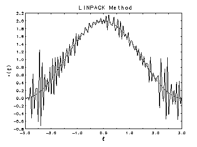
The plots below show two estimates of the solution to a 150 x 121
linear regression problem obtained by discretizing a well known ill-posed
problem and adding random errors obtained by sampling from
 with
with

which means that the errors in the elements of the right hand side vector
were in the 6th digit. The dashed curve in each plot is the true solution  , and
the jagged solid curve is the estimated solution.
The upper plot left was calculated in double precision with
machine epsilon = 2.22E-16, and lower one was
calculated in single precision with machine epsilon = 1.19E-7. Since the condition number of the matrix
was 2.9E+9, the conventional interpretation of the above
perturbation bound suggests that the double precision estimate should be
accurate to 6 digits, but the single precision estimate should not contain
any digits of accuracy. Yet the two are graphically identical!
 Double Precision
  Single Precision
 A statistical perturbation analysis of the linear regression problem yields a much more realistic bound for the uncertainties in the estimated solution. The expected uncertainty in a single element of the estimate is shown to depend not on the condition number of the matrix, but rather on its smallest singular value. For the problem illustrated above, the Wilkinson perturbation approach gave

while the statistical perturbation approach gave

The latter value is much more realistic that the former, but it exceeds the true value by a factor of 2.85. Actually, the whole perturbation approach is rather irrelevant since classical regression theory provides confidence intervals for the individual elements of the estimate which modern least squares algorithms could easily compute by inverting an upper triangular matrix formed in computing that estimate. Unfortunately the numerical analysis community seems to be unaware of this fact, and the least squares subroutines in the widely used LINPACK and LAPACK collections do not return confidence intervals, or even the variance matrix needed to compute them.
For more information, see: Rust, Bert W. (1994) "Perturbation Bounds for Linear Regression Problems", (postscript, 236K bytes), Computing Science and Statistics, 26, Interface Foundation of North America, pp. 528-532.
or: "interface94.ps.gz", (zipped postscript, 68.8K bytes).
Fredholm integral equations of the first kind are used to model measurements obtained with an instrument which distorts and/or smooths the function being measured. The kernel models the instrument response function and the right hand side function models the measurements obtained. Unfortunately, real instruments also add random measurement errors to the observed right hand side. These uncertainties, no matter how small, make a stable inversion of the integral equation impossible. Small errors in the observations produce huge errors in the solution of the integral equation -- hence the name "ill-posed problems." When such a problem is discretized, in order to compute a numerical solution, the result is an ill-conditioned linear regression problem which can be made to yield physically reasonable estimates only by imposing physically motivated side constraints on the problem.
Discretizing an ill-posed problem yields an ill-conditioned
linear regression model
Least squares gives a wildly unstable estimate of
For more information, see: Rust, Bert W.,
Truncating the Singular Value Decomposition for Ill-Posed Problens
, (postscript, 2.57M bytes), NISTIR 6131, U.S. Dept. of Commerce, July 1998.
or:
MS-TruncSVD.ps.gz, (zipped postscript, 555K bytes).
The linear, first-kind integral equations which model many physical measurement
processes constitute an ill-posed problem when the measurement errors are
taken into account. When discretized, they produce ill-conditioned linear
regression models whose solutions are pathologically sensitivite to even very
small errors. Stable solutions can often be found by imposing
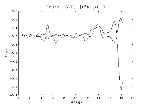
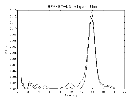
physically motivated nonnegativity constraints. Pictured below are plots of
estimated one-at-a-time, 95% confidence intervals for the flux of monoenergetic
neutrons from the nuclear reaction T (d,n) 4He. Although
the expected peak at 14 MeV is discernible in the top plot, which shows the
classical unconstrained confidence intervals, it is accompanied by three
other spurious peaks, and most of the lower bounds and some of the uppper
bounds are negative. The lower plot shows the bounds obtained when a
nonnegativity constraint is imposed on the solution. The result is a
very clean energy spectrum dominated by the expected peak at 14 MeV.
The method for computing nonnegatively constrained, simultaneous confidence
intervals has been known for some time (Burrus, W.R., Utilization of
a priori information by means of mathematical programming
in the statistical interpretation of measured distributions,
ORNL-3743, June 1965). The extension of the method to compute
one-at-a-time invtervals is described in: Rust, B.W. and O'Leary, D.P.,
"Confidence intervals for discrete approximations to ill-posed
problems," Jour. Comp. Graph. Statistics, 3 (1994) pp. 67-96.
The abstract for this paper is given below:
We consider the linear model
obtained by discretizing a system of first-kind integral equations
describing a set of physical measurements.
The n-vector
An extended version of this paper, which gives more details and includes a
real world example, can be found in: Rust, B.W. and O'Leary, D.P.,
Confidence Intervals for Discrete Approximations to Ill-Posed Problems,
NISTIR 4720, U.S. Dept. of Commerce, Jan. 1992.
It is now generally accepted that the Earth is warming because of an enhancement
of the greenhouse effect caused by increasing emissions of carbon dioxide from
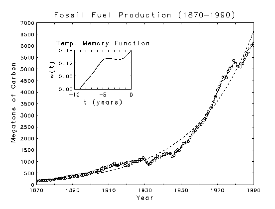
fossil fuel consumption. The circles in the plot below represent the
global, yearly fossil fuel production totals for the indicated years. The
dashed line is a nonlinear least squares fit of an exponential function to
the data. The departures of the measured values from this exponential
baseline are inversely proportional to global temperature variations. The
solid line is the fit of a model which which takes this temperature
modulation into account. This inverse modulation represents a feedback
consistent with the Gaia hypothesis for planetary greenhouse temperature
control. The model predicts that increasing temperatures will tend to
suppress the growth of fossil fuel production.
More details about this temperature modulation model are given in the paper:
Rust, B.W. and Crosby, F.J., "Further studies on the modulation of fossil
fuel production by global temperature variations," Environment
International, 20 (1994) pp. 429-456. The abstract of this paper
is given below:
We extend the earlier work of Rust and Kirk (Rust, B.W. and Kirk, B.L.,
Environment International, 7, 1982, pp. 419-422)
on the inverse modulation of
global fossil fuel production by variations in Northern Hemispheric
temperatures. The present study incorporates recent revisions and extensions
of the fuel production record and uses a much improved temperature record.
We show that the new data are consistent with the predictions of the original
Rust-Kirk model which we then extend to allow for time lags between variations
in the temperature and the corresponding responses in fuel production.
The modulation enters the new model through the convolution of
a lagged averaging function with the temperature time-series.
We also include explicit terms to account for the perturbations caused by the
Great Depression and World War II. The final model accounts for 99.84% of
the total variance in the production record. The temperature modulation
produces variations of as much as 30% in the total production. This
modulation represents a feedback which is consistent with the predictions of
the Gaia hypothesis for a planetary greenhouse temperature control. We use
the new model to calculate 20-year fuel production predictions for
three temperature scenarios which hopefully bracket the possibilities for
temperature behavior during that time.
Abstract: One argument often used against global warming is
that the global temperature record is too noisy to allow
a clear determination of the signal. This paper presents
two models for the signal which suggest that:
(1) the warming is accelerating,
(2) the warming is related to the growth
in fossil fuel emissions,
and (3) the warming in the last 146 years has been at least
10 times greater than the noise level.
One model uses a constant rate
for the acceleration and the other an exponential whose
rate constant is exactly one half that of the growth in
fossil fuel emissions. The two models can be viewed as
best case and worst case scenarios for extrapolations into
the future, but the data measured so far cannot reliably
distinguish between them.
Truncating the Singular Value Decomposition for Ill-Posed Problems

 and
a sum of squared residuals much smaller than the expected value.
Apparently the estimate captures
part of the variance that properly belongs in the residuals.
One strategy for stabilizing the estimate by
shifting some of this variance to the residuals is to truncate the
singular value decomposition
  where
where
 and
and  are orthogonal and
  is a
diagonal matrix of singular values. Singular values below some
threshold are reset to zero to give a new diagonal matrix
  ,
and the estimate is calculated from the generalized inverse of
 . The most delicate part
of this procedure is the determination of the truncation threshold.
Conventionally this has been regarded as a problem of determining the
``numerical rank'' of
  ,
but in most cases
  is clearly not rank-deficient.
This paper suggests an alternate strategy which uses the variances of the
measurement errors to specify a truncation for the elements of the vector
 . The idea is to zero the elements
dominated by measurement errors and compute the estimate using
the full rank matrix. The problem of setting the truncation threshold
becomes equivalent to deciding which of the rotated measurments are
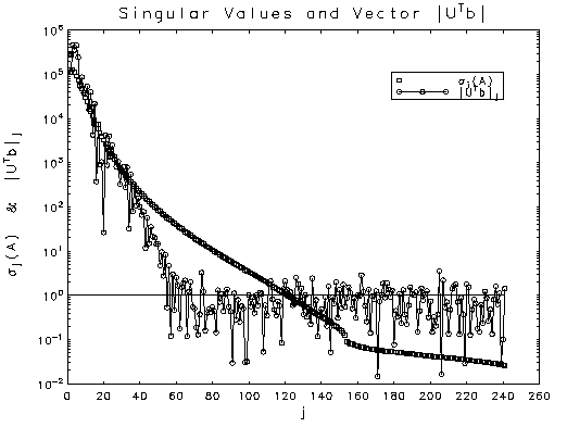
significantly different from zero. Plotted above against element number
are the singular values (squares) and the absolute values of the
elements of
  (connected circles)
for a problem which has been scaled so that the elements of
  are idependently and identically distributed with the standard normal
distribution. These values were computed with an arithmetic precision of
2.22E-16 so the matrix is clearly not rank deficient.
The dichotomy in the distribution of the elements of
 indicates the level of measuring error saturation, with the
horizontal line marking the
  level. Choosing a
truncation level of
  gives a stable estimate and an acceptable value for the sum of squared residuals.
Parameter Selection for Constrained Solutions to Ill-Posed Problems
Reprinted from
Computing Science and Statistics, Volume 32
Confidence Intervals for Discrete Approximations to Ill-Posed
Problems
 Flux unconstrained
 Flux nonnegative
 represents the desired quantities, the
m x n matrix
  represents the instrument response functions,
and the
m-vector
  contains the measurements actually obtained.
These measurements are
corrupted by random measuring errors
  drawn from a distribution with zero mean vector
and known variance matrix. Solution of first-kind integral equations is an
ill-posed problem, so the least squares solution for the above model is
a highly unstable function of the measurements, and the classical confidence
intervals for the solution are too wide to be useful.
The solution can often be stabilized
by imposing physically motivated nonnegativity constraints.
In a previous paper (O'Leary, D.P. and Rust, B.W., SIAM J. Sci. Stat. Comput.,
7, 1986, pp. 473-489) we developed a method for
computing sets of nonnegatively constrained simultaneous confidence
intervals. In this paper we briefly review the
simultaneous intervals and then show how to compute nonnegativity
constrained one-at-a-time confidence
intervals.
The technique gives valid confidence intervals even for
problems with m < n. We demonstrate the methods
using both an overdetermined and an underdetermined problem obtained
by discretizing an equation of Phillips (Phillips, D.L., J. Assoc. Comput.
Mach., 9, 1962, pp. 84-97).
Global Temperatures, Gaia, and Fossil Fuel Production
Separating Signal from Noise in Global Warming
Reprinted from
Computing Science and Statistics, Volume 35 (2003) pp. 263-277.
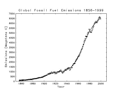 Annual Global Total Carbon Dioxide Emissions
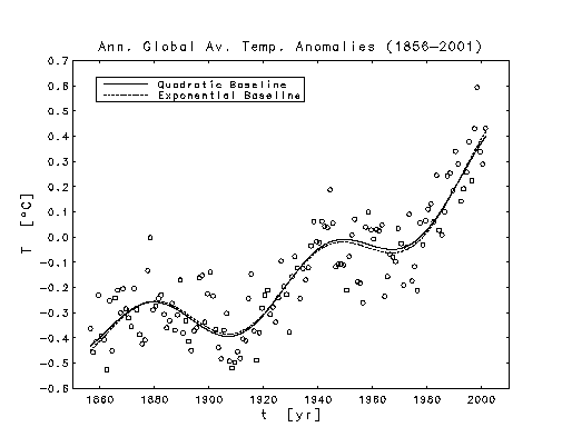 Annual Global Average Temperature Anomalies
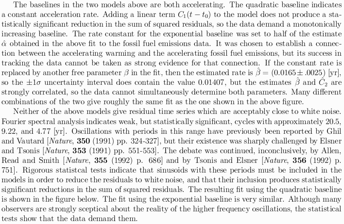
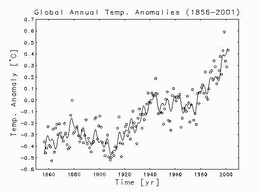 The Quadratic Baseline Fit
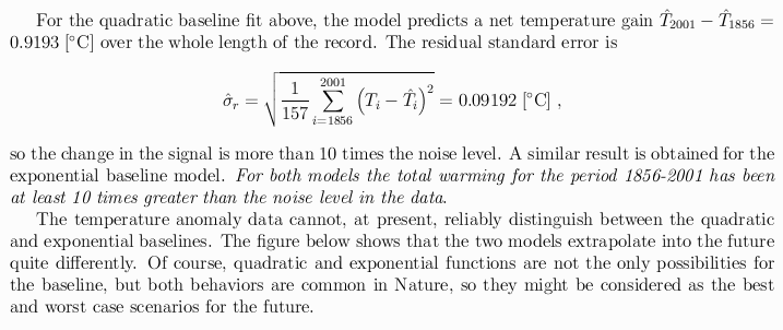
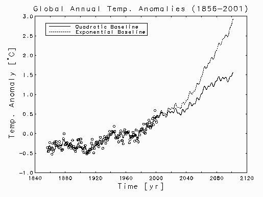 100 Year Extrapolations
Abstract: In his recent novel, State of Fear
[HarperCollins, 2004],
Michael Crichton questioned the connection between global
warming and increasing atmospheric carbon dioxide by pointing
out that for 1940-1970, temperatures were decreasing while
atmospheric carbon dioxide was increasing. A reason for this
contradiction was given at Interface 2003
[ B.W. Rust, Computing Science
and Statistics, Vol. 35 (2003) pp. 263-277 ]
where the temperature time series was well modelled by a 64.9 year
cycle superposed on an accelerating baseline. For 1940-1970,
the cycle decreased more rapidly than the baseline increased.
My analysis suggests that we are soon to
enter another cyclic decline, but the temperature
hiatus this time will be less dramatic because the baseline
has accelerated. This paper demonstrates the connections
between fossil fuel emissions, atmospheric carbon dioxide
concentrations, and global temperatures by presenting coupled
mathematical models for their measured time series.
Carbon Dioxide, Global Warming, and Michael Crichton's "State of Fear"
To be published in
Computing Science and Statistics , Vol. 37.
The plots just below have been reconstructed to look like the ones at the top of
page 86 in Michael Crichton's novel State of Fear.
It was necessary
to manually digitize the data curves in the book because he
did not cite a source for the "CO2 Levels" curve, and the sources
cited for the "Annual Mean" curve of temperature anomalies do not correspond
to the data actually plotted.
Also, the "5-year Mean" curve appears to be a plot of
11-year running means. He included these plots in order
to allow one of his characters, on page 87, to pose the question:

So, if rising carbon dioxide is the cause of rising temperatures, why
didn't it cause temperatures to rise from 1940 to 1970?
The book also contains
many other time series plots of local temperature anomalies in various
cities around the world, many of them showing definite cooling rather than
warming trends. He uses all these plots to argue that global warming is a
hoax foisted on the world by environmentalists with a secret agenda. This
message has been warmly received by some
high government officials and
conservative pundits, but has been sharply criticized by
others more familiar with the measurements.
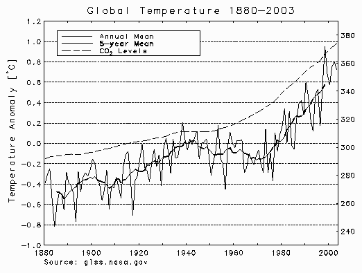 Crichton's plot on page 86
 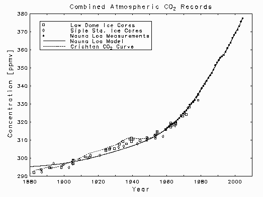 Atmospheric carbon dioxide concentrations

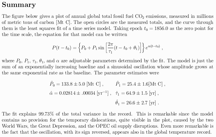
The emissions data used to define the function P(t) are plotted, in units of megatons of carbon per year, as discrete points below, where the solid curve through them is the least squares fit of the model


When the above parameter estimates were used to define the function P(t) in the above expression for c(t), the fit of that function to Keeling's atmospheric CO2 measurements gave the parameter estimates

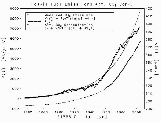 Fossil fuel emissions of carbon dioxide
 Crichton's annual global average temperature anomaly curve is replotted in the figure below. In the text he refers the reader to an Appendix where he claims that
World temperature data has been taken from the Goddard Institute for Space Studies, Columbia University, New York (GISS); the Jones, et al. data set from the Climate Research Unit, University of East Anglia, Norwich, UK (CRU); and the Global Historical Climatology Network (GHCN) maintained by the National Climatic Data Center (NCDC) and the Carbon Dioxide Information and Analysis Center (CDIAC) of Oak Ridge National Laboratory, Oak Ridge, Tennessee.In fact, his curve does not correspond to any of the annual global average data sets given by these sources. The GISS and CRU records have been plotted as discrete data points in the figure below. In each case, the reference temperature for the anomalies has been readjusted to minimize the mean square difference between the record and Crichton's curve. These zero-point adjustments brought the GISS and CRU anomalies into good agreement with one another, but neither record is concordant with Crichton's curve. There is good agreemnt in the middle of the records, particularly in the years 1940-1970, but at the beginning and end, Crichton's curve displays significant departures from all of the records which he cited as sources. In particular, his curve completely misses another period of cooling in the years 1880-1910. Had he noticed that, he might have discovered the answer to his question about the cooling in the years 1940-1970.
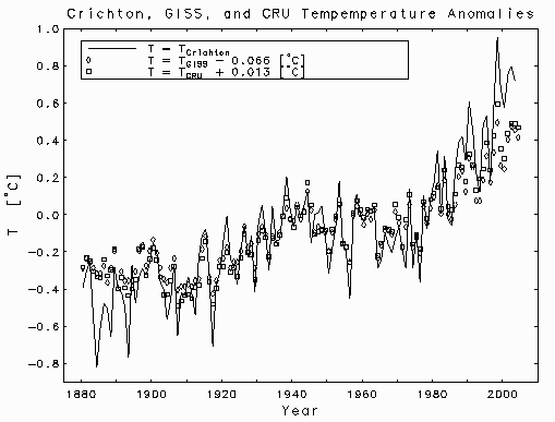 Crichton,
GISS, and
CRU
anomalies
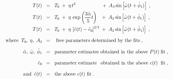
 An oscillation in the global climate system of period 65-70 years.The CRU estimates of annual global average temperature anomalies are plotted below, as discrete open circles, together with the linear least squares fits of the three mathematical models:

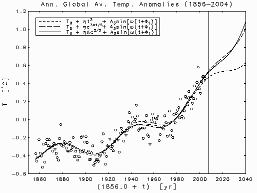 CRU's temperature anomalies
 The three accelerating baselines used in the above temperature models do not exhaust all the possibilities, but they all represent behavior that is common in nature. The quadratic baseline represents constant acceleration. Adding a linear term to that model does not produce a statistically significant reduction in the sum of square residuals, so the data seem to demand a monotonically increasing baseline.
The rate constant for the exponential baseline, &alpha &prime = 3 &alpha / 5, was chosen, somewhat arbitrarily, from the interval [0.0146 &le &alpha &prime &le 0.0190] yr -1. Changing it to any other value in that interval would work just as well because the estimate for &eta would also change in just the right way to produce almost the same fitted curve.
The most interesting of the three models is the one with the baseline given by a power law relation between changes in temperature and changes in atmospheric CO2 concentration. The power &nu = 2/3 was chosen, again somewhat arbitrarily, from the interval [0.582 &le &nu &le 0.708]. Any other value in the interval would have worked about as well, with the estimate of &eta changing in just the right way to give almost the same fitted curve.
Each of the three models explained &asymp 85% of the variance in the data, so there is no good way to choose between them. Although they give similar fits to the currently available data, they extrapolate into the future quite differently. The next maximum of the temperature cycle will occur in September 2007 and the next minimum in March 2040. Assuming that the present rate of increase in fossil fuel production can be maintained implies that the approaching cooling period will not be so pronounced as the ones that started in &asymp 1880 and in &asymp 1940. Only the constant acceleration, quadratic baseline model would produce a noticeable hiatus in the rising temperatures.
Fitting Nature's Basic Functions
This is a series of articles, published in Computing in Science and Engineering, on the art of least squares modelling of measured time series data using combinations of the most basic functions governing the dynamics of natural processes, with a particular emphasis on cyclical and exponential behavior. The modelling techniques are applied to the historical records of global total fossil fuel carbon dioxide emissions, atmospheric carbon dioxide abundance, and global average temperatures of the lower troposphere. Standard statistical diagnostics are used to assess the models and the connections between them. Short-term extrapolations into the future are considered.
This installment explains linear least squares with a special emphasis on
polynomial fits. It describes the statistical assumptions in the general
linear model and explains why the least squares calculation gives the best
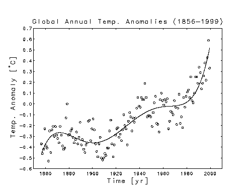
linear unbiased estimate for the unknown parameters. It uses the meaured
global average annual temperature record for the years 1856-1999 as an example
data set and shows that a polynomial of degree at least five is required to
capture the systmatic variation in the record.
Unfortunately, the final published manuscript had some errors. Corrections
can be obtained from
Errata for Part I
This installment explains statistical diagnostic techniques for
evaluating linear least squares fits. Topics covered include the variance
and correlation matrices for the least squares estimate, construction of
confidence intervals for the estimate, and testing hypotheses about the
statistical significance of the individual components of the estimate. The
use of the techniques is illustrated by applying them to the analysis of
polynomial fits to the meaured global average annual temperature record for
the years 1856-1999. In particular it is shown that for a quadratic polynomial
fit, the coefficient of the linear term is not statistically significant.
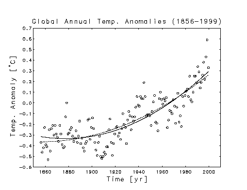
The solid curve in the plot below represents a full quadratic fit, with
three adjustable paramenters, and the dashed curve represents a reduced
quadratic fit, with the parameter for the linear term omitted. Including
the linear parameter does not produce a statistically significant reduction
in the is sum of squared residuals. This suggests that the baseline trend
for the global warming is increasing monotonically.
This installment introduces nonlinear least squares fitting and
describes the Gauss-Newton iteration and the Levenberg-Marquardt variant of it.
It explains how to fit exponential and sinusoidal functions to measured data
and how to compute statistical diagnostics and test hypotheses about the fits.
It illustrates the techniques by fitting various nonlinear models to the
the time series records of annual global total fossil fuel emissions
for the years 1751-1998 and global annual average temperatures for 1856-2001.
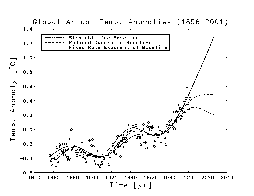
All of the curves in the plot below were
obtained by nonlinear least squares fitting of models with 5 adjustable
parameters. In each case, three of the parameters defined a sinusoid with
a period of approximately 65 years. The other two parameters defined a
baseline. The reduced quadratic baseline had the same form as the one
discussed in Part II. The fixed rate exponential baseline had the form
of a constant plus an exponential whose rate was fixed at the value obtained
from the above exponential fit to the fossil fuel emissions data. All of
the terms in the 3 fits were statistically significant. The straight line
baseline fit accounted for 75.8% of the total variance in the data, the
exponential baseline fit accounted for 79.0%, and the reduced quadratic
baseline fit accounted for 81.0%.
Fitting Nature's Basic Functions Part I: Polynomials and
Linear Least Squares
 The Temperature Data
Fitting Nature's Basic Functions Part II: Estimating Uncertainties and
Testing Hypotheses
 Temperature Data (same as in Part I)
Fitting Nature's Basic Functions Part III: Exponentials, Sinusoids, and
Nonlinear Least Squares
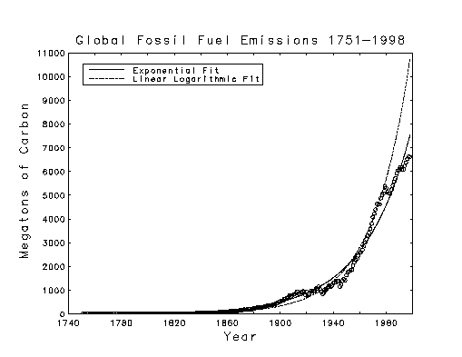
The linear logarithmic curve above was obtained from a linear least squares
fit of a straight line to the logarithms of the data, and the exponential curve
was obtained by nonlinear least squares fitting to the data itself. Both fits
used 2 adjustable parameters.
 Fossil Fuel Emissions Data
  Temp. Data (different from Parts I & II)
Fitting Nature's Basic Functions Part IV: The Variable Projection
Algorithm
 Fossil Fuel Emissions Data (Different from Part III)
 Temp. Data (Same as in Part III)