Part dimensions: 500 nm x 200 nm x 0.6 nm
Ms=1.1e6 A/m, A=1.6e-11 J/m
K1=5.1e5 J/m3 along the (0,0,1) axis
DMI: D=3.5e-3 J/m2, Free boundaries
Use
the Oxs_DMExchange6Ngbr
extension to model the DMI.
Initial magnetization configuration:
Ignoring z-coords, let P be the
point (50 nm, 50 nm) relative to the lower left hand
corner of the simulation. Set m=(0,0,1) for all points closer to P
than 16 nm. Set m=(0,0,-1) for all points farther from P than
23 nm. For points in-between, set m to point towards P. Write a
Tcl proc to use with Oxs_ScriptVectorField
to set up this initial configuration. This initial configuration is
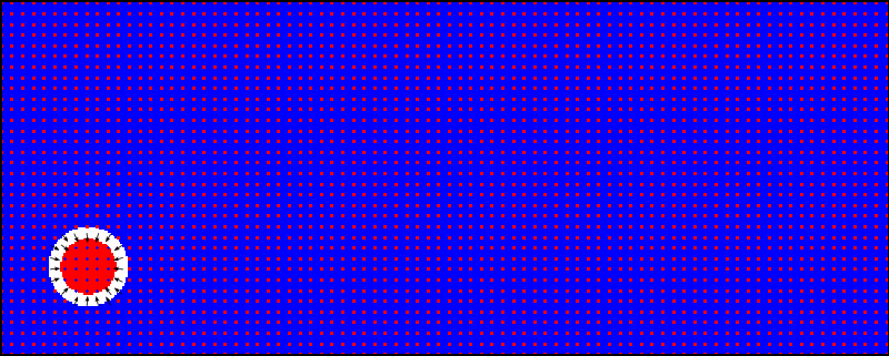
illustrated below. Initial magnetization. Background color indicates z-component of
magnetization, with red indicating out of plane (z>0), blue
is into plane (z<0), and white is in plane
(z=0).
Relax to equilibrium:
Use Oxs_CGEvolve
to relax the initial state towards equilibrium. Try different cell
sizes in the range 1 nm to 4 nm. The magnetization should relax into
a skyrmion. If the skyrmion forms but wanders away from the initial
location, introduce a small region with larger K1 near P to pin the
skyrmion. See how small K1 needs to be to hold the skyrmion in
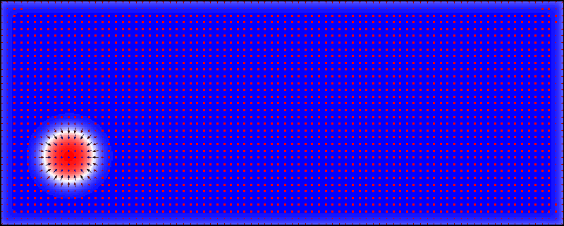
place. The equilibrium state should be similar to the following two figures.
Equilibrium magnetization. As above, background color
indicates z-component of magnetization, with red indicating
out of plane (z>0), blue is into plane
(z<0), and white is in plane (z=0).Anisotropy energy density in equilibrium configuration. Background
color indicates magnitude of energy density, where orange is
≈500 kJ/m3 and green is close to zero.
In the next session we will introduce a spin current to move the
skyrmion.
 OOMMF Tutorial Series: Homework