 OOMMF Tutorial Series
Addendum: Skyrmion Tracking
OOMMF Tutorial Series
Addendum: Skyrmion Tracking
At times one would like to extract from a micromagnetic simulation
the position of a particular feature, such as a domain wall or a
vortex, and track the motion of that feature as a function of time
across the simulation run. Automated feature detection is very
difficult in general, but there are some simple special cases. For
example, the location of a head-to-head domain wall in a horizontal
strip can be deduced from the x-component of the average magnetization
(cf. D.G. Porter and M.J. Donahue, “Velocity of transverse
domain wall motion along thin, narrow strips,”
Journal of Applied Physics, 95, 6729-6731 (2004). DOI:
10.1063/1.1688673), and vortex positions in square plates can be
computed from the x- and y-components of average magnetization (as
in µMAG
Standard Problem #5).
This page presents a straightforward method for tracking the
motion of a skyrmion across a thin plate, as illustrated in this video
based on the OOMMF tutorial session 3
homework problem:
The key point of the method is the observation that the spins inside the skyrmion bubble point out of the plane of the film (mz>0) while the rest of the spins point into the plane (mz<0). Since the skyrmion is circular, we can estimate the center of the skyrmion by averaging the locations of all spins with mz>0.
Skyrmion Simulation
The simulation above was creating by running the OOMMF boxsi solver first on skyrmion_example‑init.mif to find the zero-current equilibrium magnetization state, and then using that as the initial state along with a constant effective current density J P = 1.4×10¹² A/m2 (u = 100 m/s) in skyrmion_example.mif. The simulations rely on the OOMMF extension anv_spintevolve to model the spin-torque effect and DMExchange6Ngbr to include the Dzyaloshinsky-Moriya interaction. (Both extensions are included in standard OOMMF distributions.)The second simulation writes the magnetization spin configuration to disk at simulation time intervals of 50 ps, with file names
- skyrmion_example‑alpha0.100‑Oxs_TimeDriver‑Spin‑00‑0000000.omf
- skyrmion_example‑alpha0.100‑Oxs_TimeDriver‑Spin‑00‑0000157.omf
- skyrmion_example‑alpha0.100‑Oxs_TimeDriver‑Spin‑01‑0000317.omf
- skyrmion_example‑alpha0.100‑Oxs_TimeDriver‑Spin‑02‑0000477.omf
- skyrmion_example‑alpha0.100‑Oxs_TimeDriver‑Spin‑03‑0000637.omf
- …
- skyrmion_example‑alpha0.100‑Oxs_TimeDriver‑Spin‑77‑0012477.omf
- skyrmion_example‑alpha0.100‑Oxs_TimeDriver‑Spin‑78‑0012637.omf
- skyrmion_example‑alpha0.100‑Oxs_TimeDriver‑Spin‑79‑0012797.omf
Tracking Skyrmion Location
The first (and key) step in processing the spin configuration files is to pass them through the OOMMF command line program avf2odt. This program reads magnetization and other vector field files and writes derived data in a plain text tabular format. The command for this example istclsh oommf.tcl avf2odt -average space \
-index t ns '$i*0.05' \
-valfunc xpos nm '$vz>0.5 ? $x*1e9 : 0' \
-valfunc ypos nm '$vz>0.5 ? $y*1e9 : 0' \
-valfunc wgt '' '$vz>0.5 ? 1 : 0' \
-defaultvals 0 -headers collapse -truncate 1 -onefile foo-a.odt \
skyrmion_example-alpha0.100-Oxs_TimeDriver-Spin-*omf
\’. On Windows either merge all the lines
together onto one line, or else replace the backslash characters with
the Windows continuation character ‘^’. On
Windows you will also need to replace the single quotes with double
quotes throughout. I give now a brief overview of the avf2odt options
used above; see the avf2odt documentation for additional details.
The back end of the command lists all the files we want to
process, namely all of the files output from the simulation.
Each file will correspond to one row in the output table, processed in
the order given on the command line. Glob string matches
(* and ?) will be sorted in alphabetical
order. By default avf2odt will print to stderr the name of each file
as it is processed. (This logging can be suppressed with
the ‑v 0 option.)
Moving to the front of the options list, we see
the ‑average specification. avf2odt condenses data in a
vector field file by computing averages across a sequence of
regions. For example, you can request averages across lines or planes
parallel or perpendicular to coordinate axes to create line profiles
and cross-sectional averages. In this instance we want to average
spins across the 3D volume, so we specify ‑average
space.
Next we specify what output we want. We want a time index for each
snapshot, so we use ‑index t ns '$i*0.05',
where ‑index indicates values determined by the
sequential processing order of the files. The first two
subfields, t and ns, specify the column title
and units (here “t” for time and “ns” for
nanoseconds). The third subfield is a Tcl expr expression for the values
to put into the column, where $i is the 0-based index of
the file being processed. Our output files are spaced 50 ps apart,
so the expression '$i*0.05' will convert the file index
number into a time index in nanoseconds. A side note: On unix it is
critical to enclose the expr expression in single quotes, as otherwise
the unix shell will try to perform variable interpolation and wildcard
expansion at the $ and * characters,
respectively.
The ‑valfunc items are the key bits in the skyrmion
identification. As in the ‑index option, the first
two subfields specify the column name and units in the output table, and
the third subfield is a Tcl expr expression for the column values. The
primary variables available in this expression
are $x, $y, $z and
$vx, $vy, $vz representing the
three location coordinates and three field coordinate values at each
point in the file. The Tcl expr expression is evaluated once for each
point in the file, and the average value is output to the table row
corresponding to the file.
The expression '$vz>0.5 ? $x*1e9 : 0' uses the ternary
operator to check a condition ($vz>0.5), and if true
returns the the x-coordinate of the point multiplied by 109
(a convenience, to convert from meters to nanometers), and if false
returns 0. In this way we average the x-coordinates of only points
inside the skyrmion, as indicated by having z-component of spin (in
this context mz is $vz) larger than
0.5.
Two important notes: First, if the skyrmion center were pointing into
the plane instead of out, then the test should
be $vz<-0.5 instead of $vz>0.5. Second,
if we were processing a magnetization file instead of a spin file, we
would want to compare $vz to say half the saturation
magnetization instead of 0.5. In particular, if your simulations have
regions where Ms = 0, then you should work with
::Magnetization files instead of ::Spin files because the latter will
have randomly oriented spins in the Ms = 0 regions
which may be difficult to exclude from the averaging process.
There is a similar expression in the next line of the command to
collect the average y-coordinate of points inside the skyrmion,
followed by
‑valfunc wgt '' '$vz>0.5 ? 1 : 0'. This expr
expression simply tallies the number of points we are counting
inside the skyrmion, so we can properly normalize the results in the
next step.
The remaining options merely request no data table columns other than
the ones we've expressly requested (‑defaultvals
0), collect all the data together into a single file named
foo‑a.odt (‑headers collapse ‑onefile
foo‑a.odt), and overwrite foo‑a.odt if it already
exists (‑truncate 1).
The output produced by this command, stored in the file foo‑a.odt, has this form:
# ODT 1.0
## Desc: Data from 81 vector field files: skyrmion_example‑init.omf,
...
# Columns:\
#        t                  xpos               ypos               wgt
#  Units:\
#        ns                  nm                 nm                 {}
 0.00000000000000    0.603560000000000  0.603560000000000  0.0105200000000000
 0.0500000000000000  0.644760000000000  0.603000000000000  0.0104400000000000
 0.100000000000000   0.718200000000000  0.627400000000000  0.0107600000000000
 0.150000000000000   0.774960000000000  0.639680000000000  0.0108000000000000
...
 3.90000000000000    4.72972000000000   1.13836000000000   0.0109200000000000
 3.95000000000000    4.73040000000000   1.13400000000000   0.0108000000000000
 4.00000000000000    4.78200000000000   1.14344000000000   0.0108000000000000
# Table End
We are now almost done. The first column contains the time index for
each file, in nanoseconds. But the second and third columns, xpos and
ypos, are not the skyrmion center, but rather some normalized sum of
the locations of the spins inside the skyrmion. To get the skyrmion
center coordinates we need to divide the xpos and ypos values in each
row by the corresponding value in the last column. If you wish you can
import this file into your favorite spreadsheet and implement the
conversion there. An alternative is to use the OOMMF command
line tool
odtcalc. We
will use this in conjunction with the OOMMF command line tool
odtcols
to get our final results:
tclsh oommf.tcl odtcalc x '$xpos/$wgt' nm y '$ypos/$wgt' nm < foo-a.odt > foo-b.odt
tclsh oommf.tcl odtcols t x y -f '%10.3f' < foo-b.odt > skyrmion-position.odt
odtcalc command takes parameter triples similar in format to
the ‑index and ‑valfunc options
to avf2odt, except that the triplet order is column name,
Tcl expr expression, value units. The available variable names
come directly from the input data table column names. The output from
odtcalc repeats all the columns from the input, supplemented with an
additional column for each command line parameter triple. We only care
about the time and normalized skyrmion center locations
(columns t, x, and y, respectively), so we use odtcols
to extract just those three columns and write the result to the output
file skyrmion‑position.odt. The final result is
# ODT 1.0
## Desc: Data from 81 vector field files: skyrmion_example‑init.omf,
...
# Columns: \
# t               x               y
# Units: \
# ns              nm              nm
       0.000          57.373          57.373
       0.050          61.759          57.759
       0.100          66.747          58.309
       0.150          71.756          59.230
...
       3.900         433.125         104.245
       3.950         438.000         105.000
       4.000         442.778         105.874
# Table End
See the odtcols documentation if you want the last file
in CSV format, or as bare data with no headers.
The three commands avf2odt, odtcalc,
odtcols, can be piped together as a single command. A
slightly more sophisticated, single command version of the above is
tclsh oommf.tcl avf2odt -average space        \
  -region 12e-9 12e-9 - 488e-9 188e-9 -       \
  -index t ns '$i*0.05'                       \
  -valfunc xpos nm '$vz>0.5 ? $x*1e9*$vz : 0' \
  -valfunc ypos nm '$vz>0.5 ? $y*1e9*$vz : 0' \
  -valfunc wgt '' '$vz>0.5 ? $vz : 0'         \
  -defaultvals 0 -headers collapse -v 0 -onefile - \
  skyrmion_example-alpha0.100-Oxs_TimeDriver-Spin-*omf \
 | tclsh oommf.tcl odtcalc x '$xpos/$wgt' nm y '$ypos/$wgt' nm \
 | tclsh oommf.tcl odtcols t x y -f '%10.3f' > skyrmion-position.odt
tclsh oommf.tcl avf2odt -average space        ^
  -region 12e-9 12e-9 - 488e-9 188e-9 -       ^
  -index t ns "$i*0.05"                       ^
  -valfunc xpos nm "$vz>0.5 ? $x*1e9*$vz : 0" ^
  -valfunc ypos nm "$vz>0.5 ? $y*1e9*$vz : 0" ^
  -valfunc wgt "" "$vz>0.5 ? $vz : 0"         ^
  -defaultvals 0 -headers collapse -v 0 -onefile - ^
  skyrmion_example-alpha0.100-Oxs_TimeDriver-Spin-*omf ^
 | tclsh oommf.tcl odtcalc x "$xpos/$wgt" nm y "$ypos/$wgt" nm ^
 | tclsh oommf.tcl odtcols t x y -f "%10.3f" > skyrmion-position.odt
avf2odt command we use the
‑region option to ignore a 12 nm margin around
the outside of the simulation, in case any spins on the edge of the
simulation happen to have positive z-component and adversely impact
our skyrmion selection criterion. (Note that the region dimensions are
in meters!) The ‑valfunc expressions are also
tweaked to weight locations inside the skyrmion by the strength of the
spin z-component. If you want to try this procedure yourself, you can
compare against the full output
file that was used to produce this graph: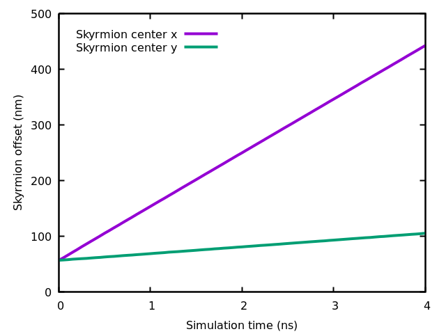
The response is linear, as expected for a constant current.
Cross-Sectional Averages
We can use the-average plane -axis x option
to avf2odt to average magnetization component values
across planes perpendicular to the x-axis. We run this on a
single file (say the 2 ns snapshot) to create a 1D collection of
averages indexed by the x offset:
tclsh oommf.tcl avf2odt -average plane -axis x \
  skyrmion_example-alpha0.100-Oxs_TimeDriver-Spin-40-*omf
-onefile, there will be one data table file
written for each input file (in this case, one file), named by
replacing the .omf extension on the input file name
with .odt. The output file has the form
# ODT 1.0
## Desc: Data from vector field file skyrmion_example-alpha0.100-Oxs_TimeDriver-Spin-40-0006557.omf
...
# Columns:\
#         x                   m_x                  m_y                  m_z
#   Units:\
#         m                    {}                   {}                   {}
  1.30000000000000e-08 -0.0666609440209170   0.0105579739019117  -0.997642757515594
  1.50000000000000e-08 -0.0466110757564310   0.00826372276950369 -0.998798356293519
  1.70000000000000e-08 -0.0325609940391627   0.00640636195278553 -0.999365093481769
...
  4.83000000000000e-07  0.0319426902806790   0.00631023003805997 -0.999385449234615
  4.85000000000000e-07  0.0457997980175227   0.00815129360001863 -0.998836608058228
  4.87000000000000e-07  0.0656066145663459   0.0104285928185419  -0.997713831845614
# Table End
which yields this graph: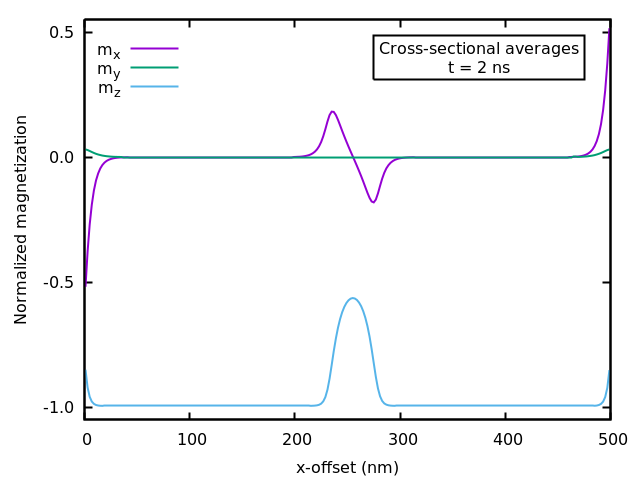
The location of the skyrmion at x = 250 nm is clearly evident in the mz trace in this graph. (Even though the mz component inside the skyrmion is greater than zero, the overall cross-sectional average is negative, just less negative in the cross-sections containing the skyrmion.) We can also see the effect of the edges of the skyrmion on the mx component, and strip edge effects in all three components at x near 0 nm and 500 nm.
Line Profiles
Use the-average point option
to avf2odt to extract raw, non-averaged data from the
.omf file. The command
tclsh oommf.tcl avf2odt -average point \
  -region - 80e-9 - - 82e-9 - -opatsub -linegraph.odt \
  skyrmion_example-alpha0.100-Oxs_TimeDriver-Spin-40-*omf
# ODT 1.0
## Desc: Data from vector field file skyrmion_example-alpha0.100-Oxs_TimeDriver-Spin-40-0006557.omf
## Active volume: (0,8e-08,0) x (5e-07,8.2e-08,6e-10)
## Cell size: 2e-09 x 2e-09 x 6e-10
## Cells in active volume: 250
#
# Table Start
# Title: Points in specified volume
# Columns:\
#         x                    y                    z                   m_x                  m_y                  m_z
#   Units:\
#         m                    m                    m                    {}                   {}                   {}
  1.00000000000000e-09  8.10000000000000e-08  3.00000000000000e-10 -0.525758122122242    0.0309270756741152  -0.850071710511967
  3.00000000000000e-09  8.10000000000000e-08  3.00000000000000e-10 -0.383855427027902    0.0282436687337109  -0.922961161868520
  5.00000000000000e-09  8.10000000000000e-08  3.00000000000000e-10 -0.274898635848724    0.0244118972955306  -0.961163253188002
 ...
  4.95000000000000e-07  8.10000000000000e-08  3.00000000000000e-10  0.272353405599773    0.0242234134112282  -0.961892326978916
  4.97000000000000e-07  8.10000000000000e-08  3.00000000000000e-10  0.381001948797025    0.0280470578610357  -0.924148731297192
  4.99000000000000e-07  8.10000000000000e-08  3.00000000000000e-10  0.522878350430820    0.0307238099376666  -0.851853437014642
# Table End
Compare the resulting graph to the previous one of cross-sectional
averages: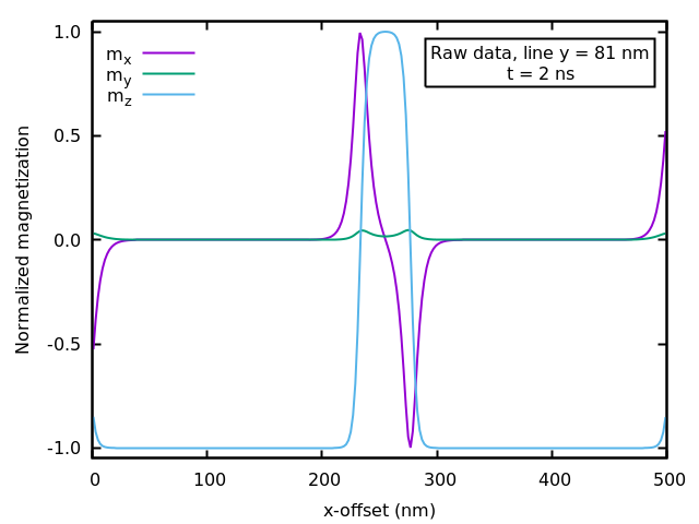
OVF File General Information
Theavf2ovf -info command can be used to
extract general information, such as extents and lattice parameters, from an OVF file:
$ tclsh oommf.tcl avf2ovf -info skyrmion_example-alpha0.100-Oxs_TimeDriver-Spin-40-0006557.omf
File: skyrmion_example-alpha0.100-Oxs_TimeDriver-Spin-40-0006557.omf
File size: 600889 bytes
Mesh title: Oxs_TimeDriver::Spin
Mesh desc---
: Oxs vector field output
: MIF source file: skyrmion_example.mif
: Iteration: 6557, State id: 45741
: Stage: 40, Stage iteration: 159
: Stage simulation time: 5e-11 s
: Total simulation time: 2.05e-09 s
Rectangular mesh
 Mesh size: 25000
 Dimensions: 250 100 1
 Value magnitude span: 0.99999999999999978 [(1.54259e-05,-4.50696e-05,-1) at (4.41e-07,5.3e-08,3e-10)]
                    to 1.0000000000000002 [(-6.58496e-11,0.525491,-0.850799) at (3.79e-07,1.99e-07,3e-10)] (in )
 Data range: (1e-09,1e-09,3e-10) x (4.99e-07,1.99e-07,3e-10) (in m)
 Mesh range: (0,0,0) x (5e-07,2e-07,6e-10) (in m)
 Mesh base/step: (1e-09,1e-09,3e-10)/(2e-09,2e-09,6e-10) (in m)
This can be useful for range selection when constructing
avf2odt commands.
Back to OOMMF Tutorial
Date created: February 9, 2021 | Last updated: February 14, 2021 Contact: Webmaster