 Movies
This page presents some movies of micromagnetic simulations of
µMAG
Standard Problem 4 using the OOMMF 3D solver Oxsii. This is an
update of an earlier
page with movies of simulations produced by the OOMMF 2D solver
mmSolve2D.
Problem discussion
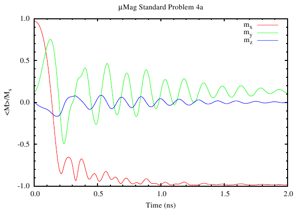
In this problem a 500 nm × 125 nm × 3 nm rectangular prism of Permalloy, initially in an equilibrium zero-field ‘S’-state, is subjected to one of two reversing fields; the reversing fields are spatially uniform with a unit step function time profile turned on at time t=0 ns.For problem part (a) the applied field is µ0H = (-24.6 mT, 4.3 mT, 0.0 mT), where the first (x) coordinate is the long (500 nm) axis of the part and the last (z) coordinate is the short (3 nm) axis. This field is in the xy-plane with of a magnitude of approximately 25 mT directed 170° from the positive x-axis. The reversal proceeds relatively smoothly with the magnetization as a whole rotating counterclockwise towards the reversed direction. The reversal overshoots before gradually settling down into the reversed (non-zero field) equilibrium state.
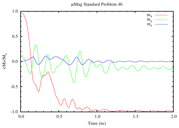
In problem part (b) the applied field is µ0H = (-35.5 mT, -6.3 mT, 0.0 mT), which has magnitude of approximately 36 mT directed 190° from the x-axis in the xy-plane. The reversal in this case is more complicated. The end regions initially rotated counterclockwise while the middle section rotates clockwise, with the result that 360° domain walls form between the middle and end domains. The 360° domain walls gradually move out from the center and dissipate at either end of the part.
Simulation details
Three OOMMF MIF 2.1 problem description files are used in these simulations. The first, stdprob4-init.mif, uses conjugate-gradient minimization to find the initial zero-field equilibrium state used as the start point for the dynamic simulations. Then stdprob4a.mif and stdprob4b.mif use a Runge-Kutta-Fehlberg 5(4) method to compute the reversal dynamics for problems part (a) and (b), respectively. The only difference between stdprob4a.mif and stdprob4b.mif is the direction and strength of the applied field. These MIF files could easily be combined into one file differentiated by a run-timeParameter,
but for simplicity of presentation that has not been done here.The discretization cell size in these simulations is set at 1 nm × 1 nm × 1 nm , so the the number of cells in the simulation is 500 × 125 × 3 = 187500 cells. This mesh is sufficiently small to keep the maximum angle between neighboring cells below about 6° in part (a) and 18° in part (b). These files are loaded into Oxsii; in the dynamic simulations the magnetization state was written to disk at the end of each stage, i.e., every 4 picoseconds of simulation time. These simulations each run 2 ns, so including the initial state 501 magnetization files are saved for each simulation.
Here are plots showing how the magnetization components,
averaged across the entire volume, vary with time:
Making movies
The first step in creating animations from the simulation output is to convert the magnetization output files into a common bitmap image format. This can be accomplished using the OOMMF command line tool avf2ppm, and the command line
tclsh oommf.tcl avf2ppm stdprob4*omf -config stdprob4-div.config \

    -opatexp "Oxs_TimeDriver-Magnetization-([0-9]+)-.*.omf" \

    -opatsub "\1.png" -filter pnmtopng
File|Write config…
dialog box in mmDisp, and then additional edits are made with a
plain text editor. In particular, the configuration options
   arrow,antialias           1

   misc,width                1200

   misc,height               360

   misc,crop                 0
The -opatexp and -opatsub expressions shorten
the output filenames and change the extensions to .png, e.g.,
stdprob4a-Oxs_TimeDriver-Magnetization-0000013-0000977.omf → stdprob4a-0000013.pngIn particular, this retains the stage number (here 13) and drops the iteration number (977).
The -filter pnmtopng option sends the PPM bitmap output
from avf2ppm through
the NetPBM
command line program pnmtopng, which converts the output to PNG format.
The movie making software FFmpeg can read PPM files directly, so this
step is optional. However, the (compressed) PNG files are much smaller
than the (uncompressed) PPM files, so this step reduces intermediate disk
space usage.
Once the bitmap files are created, the FFmpeg tool can be used to create movies in any of a wide variety of formats. For this page movies are made in three formats: MP4, WebM, and Ogg. (FFmpeg can also be used to create animated GIFs. However, they can be rather large, so for performance reasons the instructions for building animated GIFs are on a separate page.)
The commands for creating the Standard Problem 4a movies are
ffmpeg -start_number 0 -i stdprob4a-%07d.png -r 25 -c:v libx264 \

    -pix_fmt yuv420p -qmin 0 -qmax 32
 -an stdprob4a-div.mp4


ffmpeg -start_number 0 -i stdprob4a-%07d.png -r 25 -c:v libvpx \

    -qmin 0 -qmax 32 -an stdprob4a-div.webm


ffmpeg -start_number 0 -i stdprob4a-%07d.png -r 25 -c:v libtheora \

     -qscale:v 5 -an stdprob4a-div.ogv
-qmin, -qmax, and -qscale)
produce movies of similar quality, although the file size for the last
is a considerably bigger (18 MB) than the first two (9 MB and
6 MB, respectively). The same options are used for the Standard
Problem 4b movies; in that case the resulting movie files are sized
11 MB, 8 MB, and 21 MB respectively.The movies are 501 frames long and run at 25 frames per second, so the viewing duration is 20 seconds. The simulation time is 2 ns, so each second of viewing time corresponds to 100 ps of simulation.
The movies
µMAG Standard Problem 4a:
Download Video:
"MP4"
"WebM"
"Ogg"
µMAG Standard Problem 4b:
Download Video: "MP4" "WebM" "Ogg"
DISCLAIMER: Commercial equipment and software referred to on these pages are identified for informational purposes only, and does not imply recommendation of or endorsement by the National Institute of Standards and Technology, nor does it imply that the products so identified are necessarily the best available for the purpose.
OOMMF is an experimental system. NIST assumes no responsibility whatsoever for its use by other parties, and makes no guarantees, expressed or implied, about its quality, reliability, or any other characteristic. This software was developed at the National Institute of Standards and Technology by employees of the Federal Government in the course of their official duties. Pursuant to Title 17, United States Code, Section 105, this software is not subject to copyright protection and is in the public domain.
We appreciate acknowledgment if the software is used.
Go to
start of page or
 .
.
Date created: Sep 18, 2014 | Last updated: Sep 25, 2014 Contact: Webmaster