User’s Guide

GenPatterns

Version 2.0 (For GenPatterns Version 1.6)

7/12/2000

Antti Pesonen^*

Dan Cardy

Mathematical and Computational Science Division

Information Technology Laboratory

National Institute of Standards and Technology

• Prepared under the supervision of Fern Y. Hunt as part of a 1999 ITL research initiative in Bioinformatics.
  

Disclaimer of liability

For documents and software related to GenPatterns, the authors or the U.S. Government do not warrant or assume any legal liability or responsibility for the accuracy, completeness, or usefulness of any information, product, or process disclosed.

Content

1 Introduction...................................................................................................................................................... 5

2 Hao histogram.................................................................................................................................................. 5

3 Program installation................................................................................................................................ 6

3.1 Standalone program installation................................................................................................ 6

3.2 Applet installation.................................................................................................................................. 6

4 Basic Usage.......................................................................................................................................................... 6

4.1 Running GenPatterns................................................................................................................................ 6

4.1.1 Standalone program.................................................................................................................................. 6

4.1.2 Applet........................................................................................................................................................... 7

4.2 Using control panel.................................................................................................................................. 7

4.2.1 Launching a histogram............................................................................................................................. 7

4.2.2 Comparing histograms.............................................................................................................................. 9

4.3 Operating main histogram window............................................................................................... 9

4.3.1 The Map..................................................................................................................................................... 11

4.4 Operating compare histograms window.................................................................................. 11

5 Advanced features...................................................................................................................................... 13

5.1 Viewing the sequence............................................................................................................................... 13

5.2 Changing the color set.......................................................................................................................... 14

5.3 Generating a sample sequence......................................................................................................... 14

5.4 Generating a sub-sequence frequency-count model......................................................... 15

5.5 Using gap length histograms............................................................................................................ 16

5.5.1 What is a gap length histogram ?......................................................................................................... 16

5.5.2 A gap length histogram and GenPatterns........................................................................................... 16

5.6 Using projection curves......................................................................................................................... 17

5.6.1 What is a projection curve ?.................................................................................................................. 17

5.6.2 A projection curve and GenPatterns.................................................................................................... 18

5.7 Using DNA walks........................................................................................................................................ 20

5.7.1 What is a DNA walk ?............................................................................................................................. 20

5.7.2 A DNA walk and GenPatterns............................................................................................................... 20

5.7.3 Double DNA walks.................................................................................................................................. 20

5.8 Modifying Histogram Properties..................................................................................................... 23

5.8.1 Changing the axes/ordering.................................................................................................................. 20

5.8.2 Changing the maximum level................................................................................................................ 20

6 References......................................................................................................................................................... 24

Appendix: The applet restrictions

1 Introduction

GenPatterns is a computer program that enables one to visualize DNA and RNA sequences using the Hao Histogram method, introduced by Bailin Hao [1]. Additionally, the program offers complementary tools, like sequence modeling and gap plots, to analyze DNA/RNA sequences. GenPatterns is a Java program and thus can be run on several operating system platforms.

This user’s guide introduces the features of GenPatterns. The guide is organized as follows. The next Section gives a short description of Hao Histogram. The program installation process is given in Section 3. Section 4 shows all the basic features of the program and Section 5 introduces the advanced features that are available.

Acknowledgement: Antti Pesonen and Fern Hunt wish to thank Joseph Hubbard for telling Hunt about DNA walks, gap plots and references and also thank Jack Douglas for giving us reference [5].

2 Hao histogram

The Hao histogram is a specialized model for representing frequencies of sub-sequences of a long string of letters from the four letter alphabet A, C, G and T. The basic element of a Hao histogram is a 2 by 2 matrix (see the Figure 1). Each position of the matrix represents a single letter of the alphabet.

The alphabet of a DNA sequence is {A=adenine, C=cytosine, G=guanine, T=thymine}. The ordering of the letters in the Hao histogram is the following:

Figure 1. A basic element of the Hao histogram.

Note that in case of an RNA sequence, T is replaced with U (=uracil). If the frequencies are placed in the positions of the corresponding letter, we call the result the Hao histogram. The histogram in Figure 1 is called the first level histogram (length of each sub-sequence is one). The first level histogram only gives us a tool to visualize single letter sub-sequences of the original sequence. There are 4^K different strings of length K made of four letters. To visualize all of these strings we form a 2^K by 2^K matrix by taking a direct product (Kronecker product) of K identical basic elements of the Hao histogram. In the figure 2 we show a Hao histogram visualizing all DNA strings of length two.

Figure 2. A Hao histogram of the sequences of length two.

We call a Hao histogram, visualizing the strings of length K, the Kth level histogram. So, Figure 2 indicates the positions of the two letter frequencies in the second level histogram.

We still have to visualize the actual frequencies. Basically, we have three methods to select from: numbers, shapes and colors. We could write the actual frequencies as values inside each slot in the matrix. This would require space and thus limit too much the matrix size we can visualize on the screen. Using different shapes for different frequency intervals have the same space problem as numbers. So, colors are selected to visualize different frequency values.

Note: In the program you do not have to accept the default order of GCAT (reading across). You can set any order you want by selecting Axes from the Edit menu (see 5.8.1 ‘Changing the axes/ordering’).

3 Program installation

The GenPatterns program is available either as a standalone Java program or as an applet. The applet version of the program has memory and access restrictions (see Appendix for details) and is essentially a demonstration program. The installation process is different for the two and thus both of them are discussed in a separate subsection.

3.1 Standalone program installation

To run a standalone Java program you need a JDK (Java Development Kit) package or a JRE (Java Run time Environment) package. Both of these packages include a Java virtual machine, which actually runs the Java program. If you do not have either of them installed in your machine, you can find one from the following Web site:

http://java.sun.com/j2se/

Download the product, run it and follow the instructions to install it to your computer. If you do not want to develop Java software yourself, JRE is the choice for you.

Finally, extract the entire contents of the GenPat.zip file to whatever directory wish. (See 4.1.1 for how to run the program.)

3.2 Applet installation

The applet version of GenPatterns can be run in any computer, having an Internet browser (e.g., Netscape Navigator or Internet Explorer) installed that supports the Java language. Any other installation effort is not needed.

The web home page of GenPatterns (containing the applet) can be found at:

http://math.nist.gov/~Fhunt/GenPatterns

4 Basic Usage

This section gives basic instructions of how to use GenPatterns. Note that the example figures in this Section showing various windows of GenPatterns are captured from the Microsoft Windows NT 4.0 environment and may look a bit different in other environments.

4.1 Running GenPatterns

GenPatterns is available as a standalone Java program and as an applet. Here are the instructions of how to run these programs.

4.1.1 Standalone program

When either JDK or JRE is installed in your computer, open a command prompt window. And chose one of the options below:

Option 1: Change to the directory where GenPatterns is installed (where you extracted the .zip file to) and enter the following command:

java GenPatterns

Option 2: Don’t change to the directory where GenPatterns is installed and enter the following command:

java –cp <classPath> GenPatterns

ClassPath is the full path to the directory where GenPatterns is installed.

If you chose this option 2, the program will load with a blank rectangle in the left-hand corner instead of the GenPatterns logo. No functionality is lost, however.

If you are going to use especially large data sets (> 10 000 000 bases), increasing the Java heap size for the program use is advisable. To do that, issue the following command to start the program:

java –Xmx<maxHeapSize> –cp <classPath> GenPatterns

If you have already changed the GenPatterns directory, the –cp switch becomes unnecessary.

4.1.2 Applet

The applet version of GenPatterns can be run only under an Internet browser. Open the web page at the following address:

http://math.nist.gov/~Fhunt/GenPatterns

Follow the instructions given in the web page.

4.2 Using the control panel

The control panel window is the main module of GenPatterns. The “Launch a Histogram” button can be used to open new histogram windows with given input (see 4.2.1 ‘Launching a histogram’ for details). By pressing the button “Compare Histograms” the user can initiate the histogram comparison feature of the program (see 4.2.2 ‘Comparing histograms’ for details). Clicking on the rectangle to the left of the button will bring up a dialog that changes the maximum level calculated for a new histogram (see 5.8.2 ‘Changing the maximum level’). If you use the stand-alone version of the program, the “Exit” button terminates the program including all the sub-windows created by the program. Exiting the control panel of the GenPatterns applet does not destroy or even invalidate other windows created by the program. Clicking again on the button used to start the applet will bring the control panel back. The control window of the program is shown in the figure 3.

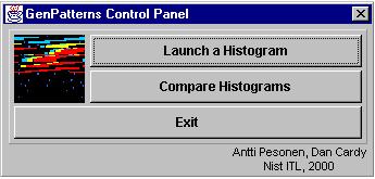
Figure 3. The control panel window.

After pressing the “Launch a histogram” button of the control panel window the user is prompted to give the full name of the input file. Both DNA and RNA sequence files are accepted as input. When running the stand-alone version of the program, a special file browse window is opened to ease the file selection task.

The format of the input file has to be one of the formats supported by GenPatterns. Thus, the input file has to be either in a FASTA format or in a special GenPatterns Frequency file (.gpf) format. The program reads the input file selected and prompts the user with a file information window (see the figure 4). The file information window gives useful details about the input file. These details include the name and the type (FASTA or GPF) / (DNA or RNA) of the file, the length of the input sequence and the number of comments and non-bases encountered in the input file. In addition to the number of comments and non-bases, also a complete list of those items with exact locations is given. Select a comment or a non-base from the list and you get the comment text or the letter of the non-base on the text area titled ‘Comment’, respectively.

The right side of the window, titled ‘The interval’, determines the interval of the original sequence. This interval is used as the actual input sequence for the Hao histogram. By default, the interval is the whole input sequence. The user can change the interval by entering new values for the Start and Stop fields. An alternative way to enter the values is to select an interval between two consecutive comments or non-bases by checking the box ‘Use selection from left’ and selecting a comment or a non-base from the list on the left.

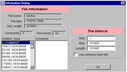
Figure 4. A file information window.

The file information in the Information Dialog window is stored to a file on the disk (the feature is disabled in the applet version of the program). The file is named adding the .fi (file information) extension to the end of the input file. An example of such a file follows:

DNA / RNA file information

==========================

FILE NAME: D:\DNAData\ecoli.fna

FILE TYPE: fasta file

SEQUENCE TYPE: DNA

SEQUENCE LENGTH: 4639221 bases + 0 non-bases

NUM OF COMMENTS: 1

====

0; gb|U00096|U00096 Escherichia coli K-12 MG1655 complete genome

====

The end of the file has a list of all the comments and non-bases found from the input file. Each entry in the list starts with the base location of the comment/non-base (0 in our example).

The file information window is accessible from the main histogram window. Select ‘File’ from the main menu and choose ‘Info...’. A similar window with the one in the Figure 4 is opened with two buttons: ‘Cancel’ and ‘Recalc’. ‘Cancel’ removes the window without any further actions. ‘Recalc’ takes the values from the interval fields ‘Start’ and ‘Stop’ and recalculates the frequency data using new input data from the interval between ‘Start’ and ‘Stop’ of the original DNA sequence.

Opening a FASTA format file starts the process of calculating the sub-sequence frequencies. This may take several minutes, depending on the length of the DNA/RNA sequence and the computer hardware. A GenPatterns Frequency file has the frequencies calculated and thus is faster to input.

After initializing proper memory structures and calculating frequencies if needed, the program creates a main histogram window to visualize the frequency data (see 4.3 ‘Operating main histogram window’ for details about the main histogram window). If no file name is given or the file entered does not have the correct format, an empty main histogram window is created.

If the input file is of the GenPatterns Frequency format, the following features of the histogram window are disabled: the gap histogram, the projection curve and the DNA walk (see the Sections 5.4 ‘Generating gap histograms’, 5.5 ‘Generating projection curves’ and 5.6 ‘Using DNA walk’ for detailed description of the features).

FASTA format

The FASTA format is a commonly used file format for storing DNA/RNA sequences. Such files are available, e.g., from the GenBank database maintained by the National Library of Medicine. The file begins with a comment line starting with the character >. The actual DNA sequence starts from the first column of the first non-comment line. Here is an example of a FASTA format file (first seven lines of the file):

>gi|868168|gb|U29055.1|MMU29055 Mus musculus G protein beta 36 subunit mRNA, complete cds

GCTTGGATTCTGAAGTGTGGAAAGCACTGAGACGTGAAGATGAGTGAACTTGACCAGCTGCGGCAGGAGG

CCGAGCAACTGAAGAACCAAATTAGAGATGCTCGTAAAGCGTGTGCCGATGCGACTCTTTCTCAGATCAC

AAACAATATTGATCCAGTGGGAAGAATCCAAATGCGGACCAGGAGAACACTGAGGGGGCATCTGGCAAAG

ATTTATGCCATGCACTGGGGCACAGACTCAAGGCTCCTTGTCAGCGCCTCTCAGGATGGAAAACTCATCA

TCTGGGACAGTTATACCACAAACAAGGTTCATGCCATCCCTCTGCGCTCCTCTTGGGTCATGACCTGCGC

ATACGCTCCTTCTGGGAATTATGTGGCCTGTGGTGGCCTGGATAACATCTGCTCCATTTACAACCTGAAA

GenPatterns Frequency-Count -format

Instead of storing the raw DNA/RNA data, the GenPatterns Frequency-count file stores the frequency-counts of sub-sequences. Its file extension is .gpf. Starting from the second line of the file, the counts are listed in a special dictionary order. The Hao order of DNA bases (G, C, A and T) makes the dictionary order special (for an RNA sequence, replace T with U). The frequencies listed first are thus G, C, A, T, following the frequencies of the sequences GG, GC, GA, GT, CG, CC, CA and so on.

There are 4^K different sequences of length K. If one of the sequences of length K is listed, all of the sequences of length K have to be listed. Keeping in mind the rule just stated, the number of frequencies listed in a GenPatterns Frequency file follows the formula å_j£k4^j, where k is the length of the longest sub-sequence of interest. An example of a file in .gpf format follows:

//GPF

348

336

353

373

94

79

104

71

30

79

120

107

82

93

89

88

141

85

40

107

In this example, the frequencies of the sub-sequences of length one and two are listed. Note, that the file begins with the comment line, starting with //.

4.2.1 Comparing histograms

Comparing histograms to each other is the second most important functionality of GenPatterns, after basic histogram visualization. Only those histograms created (opened) by the control window or by any child window of the control window, can be compared and thus, windows generated by two separate control windows can’t be compared. Pressing the “Compare histograms” button pops up the dialog window shown in the figure 5.

Figure 5. The dialog window for selecting two histograms to be compared.

The window has two lists, both of them containing the same items. The user selects one item from each list and clicks the “Compare” button to compare the histograms just selected. See Section 4.4 for details of the Compare histograms window.

4.3 Operating main histogram window

The main histogram window is the actual histogram visualization window. The window has two main parts: the histogram visualization area on the left and the Fast Selection bar on the right (see the Figure 6). Additionally, there is the histogram name bar and a color bar in the bottom of the window. The color bar shows the current color set selection used to visualize frequencies.

The standard menu bar on the top of the window offers an access to a set of tools of the program. The usage of these features is explained in this manual. Refer to the content in the beginning of this manual to find a description of each tool.

Figure 6. The main histogram window.

The histogram visualization area consists of colored boxes, each of them representing a single sub-sequence frequency. The color of a sub-sequence box is related to the frequency of the sub-sequence. The color bar under the visualization area shows the current color set of frequencies (from left to right <-> from min frequency to max frequency). The user can change the color set at will (see Section 5.1 ‘Changing the color set’).

The visualization area shows a part of the Hao histogram (a view) at a time. One can view the whole histogram or just a fraction of it. The Map feature of the program is used to navigate through the histogram (see 4.3.1 ‘The Map’, for details). The user can change the view by dragging the view with the mouse or by clicking on the Map (see 4.3.1 for details).

The Fast Selection bar has the following components:

· Histogram properties activating area

· Level selector,

· Zoom controls,

· Selected Details section (sub-sequence and its frequency),

· Query controls,

· Map activating area.

The Histogram properties activating area, which is the pink box that says Hao Histogram, is used to modify the order in which the blocks of the histogram are sorted. Click on the area to see and change the current ordering. The default ordering GCAT. See 5.8.1 ‘Changing the axes/ordering’ for more information.

The Level selector is used to select the current Hao level data shown in the histogram visualization area. The minimum level is always one and the maximum level depends on the program settings. The default is nine for the stand-alone Java program and eight for the applet. See 5.8.2 ‘Changing the maximum level’ for more information.

Zoom controls can be used to zoom in and out on the histogram visualization area. For large data sets and for higher sub-sequence levels one can focus on a specific set of sub-sequences by zooming in on a specific region of the histogram. If the visual area covers only four sub-sequence slots of the histogram, the zoom in button does not have any effect. Zooming out is the opposite operation to zoom in, thus revealing more details of the histogram. If the whole histogram is visualized (the whole histogram fits to the histogram visualization area) then pressing the Zoom out button does not have any effect.

By clicking on a histogram visualization area the user can check out the frequency-count of a specific sub-sequence. This information (the sub-sequence and its count) is printed in the Selected Details section of the Fast Selection bar. A special histogram grid is provided to ease the selection task. When the grid is activated, clicking on the histogram results printing a grid on the histogram to separate each histogram slot from the others. Additionally, the histogram slot clicked is framed with the red color. The grid feature may be turned on and off from the Edit menu (default is off).

The Query controls allow the user to obtain certain sub-sequence frequency-counts explicitly. After typing a sub-sequence in the query field and pressing the Submit button the sub-sequence and its frequency are printed in the Selected Details section.

By clicking the mouse pointer on the Map activating area, the user can activate the histogram navigation feature of the program. The functionality of the map feature is explained in the next Section.

4.3.1 The Map

The main histogram window has a special feature making it easier to navigate the histogram: the Map. The Map can be activated by moving the cursor to a specific area, titled The Map. This area is located below the Query controls on the Fast Selection bar. An example of the Map is shown in the Figure 7.

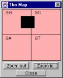
Figure 7. The Map.

The black box on the map corresponds to the current visual area of the Hao histogram on the screen. For example, the map in Figure 7 indicates that a section of sub-sequences beginning with the letter G is currently visualized on the screen – namely the sequences located in the black square. The orange region is used to orient the current visualized region within the larger portion of the histogram.

Clicking a position on the Map causes the black box to move to that position and therefore changes the visualized area of the histogram accordingly. The point the user clicks on is the new upper left corner of the visualized area.

The Map has its own zoom capability independent of the zoom capability in the visualization area of the histogram. Thus, zooming on the Map does not affect the visualized area of the histogram. Zooming in on the Map requires the black box being inside a quarter of the map area. For example, in the Figure 6 it would be impossible to zoom in because the black box crosses the line between the GG area and the GC area. Zooming out, on the other hand, would be possible in this case. Here the zoom feature can be used to select the appropriate orienting background (orange region) for a selected section of sub-sequences.

4.4 Operating compare histograms window

The compare histograms window resembles the main visualization window with a few exceptions: the Fast Selection bar is yellow and it has additional features. A picture of the compare histograms window is shown in the Figure 8. To distinguish the comparison histogram from the Hao Histogram a different color scale is used.

Figure 8. A compare histograms window.

The histogram visualization area in the figure above shows the sub-sequence frequency-count differences of two DNA sequences. The names of the input files containing the data of the sequences are printed on the bar on the bottom of the window. The order of the two input files is crucial because it determines the sign of each count difference; a sub-sequence count in the second file is subtracted from corresponding count in the first file. So, for example, the sub-sequence GTTGC with the count difference 66 in the Figure 8 states that the count of GTTGC in the input file ‘ecoli.fna’ is higher than the count of GTTGC in the file ‘SMM4_ecoli.fna’. The blue color in the matrix represents negative count differences and the red color positive differences.

The histogram comparison offers several filters to change the comparison method. The filters are ‘Log factor’, ‘Sqrt factor’ and ‘Relative count factor’. Click the checkbox with the appropriate name to activate the filter.

When the ‘Log factor’ filter is activated, instead of a frequency-count difference, a natural logarithm of the frequency ratio is calculated and visualized for each sub-sequence. For example, if we have the sequences S₁ and S₂ and their lengths are L(S₁) and L(S₂) and we also have a sub-sequence s₁ of S₁ and a sub-sequence s₂ of S₂, then we’ll get the log factored difference of s₁ and s₂ by the following formula:

(Count(s₁) / (L(S₁)-L(s₁)-1)) * ln [(Count(s₁) / (L(S₁)-L(s₁)-1)) / (Count(s₂) / (L(S₂)-L(s₁)-1))]

Note: Because of the nature of the logarithmic function, we have to take an exceptional step to be able to visualize a frequency ratio when either of the counts is zero: Both of the counts are incremented by one. If we look at the formula above, letting Count(s₂) = 0 causes a division by zero. On the other hand, letting Count(s₁) = 0 results taking a logarithm of zero which is not defined. Increasing counts is, of course, not theoretically acceptable but the correction is used for the visualization purposes only.

The square root (Sqrt) factor filter, when activated takes a square root of every scaled sub-sequence count difference before visualization. Scaling the differences means taking into account the lengths of the sequences in question. Let S₁ and S₂ be DNA sequences and let L(S₁) and L(S₂) be their lengths. Let Count_Y(X) represent the count of a sub-sequence X in the sequence Y. Then, the scaled count difference of the sub-sequence X between S₁ and S₂ is Count_S1(X) – (Count_S2(X) * ((L(S₁)-L(X)+1) / (L(S₂)-L(X)+1))), where L(X) is the length of the sub-sequence X. The scaled sub-sequence difference is calculated in every case except when the ‘Log factor’ filter is activated.

When activated the ‘Relative count factor’ takes into account the relative difference of the two counts. The factor is calculated using the following formula: 1 – (Count_S1(X) / Count_S2(X)), when Count_S1(X) < Count_S2(X). If Count_S1(X) > Count_S2(X) the formula is 1 - (Count_S2(X) / Count_S1(X)). Finally, the count difference is multiplied by the factor. The bigger the relative difference the more intense color the sub-sequence gets on the matrix. The ‘Relative count factor’ can not be used with ‘Log factor’.

A compare histogram window is equipped with a mouse click sensitive area titled “Details”. Clicking the mouse on top of the area activates a detail window that gives more detailed information on the compared sub-sequences than the main comparison window. A picture of the detail window follows.

Figure 9. A compare details window.

In addition to the information in the main comparison window, the sequence length of both compared sequences and the sub-sequence counts are given. The bottom of the window has a drop down list of Kullback-Liebler [2] values, which give the exact divergence between the compared sequences in given levels listed. The levels listed are all the levels from 1 to the set maximum level. Creating a comparison histogram window does not automatically result calculating the Kullback-Liebler values. The values are added only as the levels are visited on the compare histogram window. The “Log factor” filter has to be activated to calculate the values.

5 Advanced features

In this Section we will turn to more advanced features of GenPatterns. The features include

· viewing the base sequence,

· changing the color set of the sub-sequence frequencies,

· generating sample sequences and sub-sequence frequency models,

· using gap histograms and projection curves,

· using DNA Walk tool,

· selecting the order in which the Hao histogram is sorted.

Note that the example figures in this Section showing various windows of GenPatterns are captured from the Microsoft Windows NT environment and may look a bit different in other environments.

5.1 Viewing the sequence

To view the input DNA / RNA sequence, select ‘The sequence’ from the ‘File’ menu. The following figure gives an example of a sequence window.

Figure 10. The sequence window.

The window shows always 800 bases of the sequence at a time. The starting location of this window can be adjusted by entering a new starting location in the numeric spinner field below the sequence. Press ‘Recalc’ after entering a new value. The stop location of the window is updated automatically. The window location can also be changed by using the controls labeled ‘<<’ and ‘>>’. The ‘<<’ button moves the window 800 bases left on the sequence while ‘>>’ moves the window 800 bases right.

5.2 Changing the color set

GenPatterns uses colors to visualize the frequency-counts of sub-sequences. In principle, we could have a separate color for each count. In practice, however, the set of different colors is limited to at most 64 colors. Nevertheless, these colors can be selected from the color map of thousands of colors (if the operating system is capable of showing all of them).

Changing the color set is made easy in GenPatterns. Select ‘Edit -> Colors...’ from the main menu to get the window shown in the Figure 11.

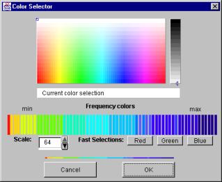
Figure 11. The color selector window.

The current (active) color set is shown under the title ‘Frequency colors’. This bar of frequency colors is divided to separate parts, each of which represents a separate interval of the original frequency-count distribution. To get the exact details of an interval, just move the cursor on top of that interval and an interval detail window will pop up to show the details. Such a window is shown in the Figure 12.

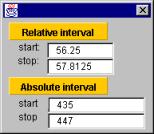
Figure 12. A color interval detail window.

The relative interval shows the relative start and ending location of the interval in percent while the absolute interval shows the minimum and maximum counts of the selected range.

To change the color of an interval first, select an appropriate color from the color map located on the top of the color selector window and then click on one of the colored bands in the strip labeled ‘Frequency colors’. Selecting a color from the color map is easy: Click on the color map on some location and the color you just clicked on is changed to be the current color. The current color is shown on the bar titled ‘Current color selection’. You can change the brightness of the selected color by clicking on the brightness bar, which is located on the right side of the color selection area (the vertical bar).

You can change the size of each interval of the color interval bar. It’s done by changing the ‘Scale’. The maximum (and the default) scale is 64 intervals. The minimum scale is 2 intervals.

The color selector window has three ‘Fast Selection’ buttons, labeled ‘Red’, ‘Green’ and ‘Blue’. Press one of these buttons to change the whole color set to represent different intensities of the color selected.

GenPatterns saves color sets of every DNA/RNA sequence to the directory the input data of the sequence was loaded from. This process is fully automatic and invisible to the user. In practice, the saving is done when the visualizing window is terminated. Note that the color set saving feature is disabled in the applet version of the program.

5.3 Generating a sample sequence

GenPatterns is equipped with a sample sequence generator. By using the generator the user can generate artificial DNA/RNA sequences based on an existing DNA/RNA sequence and its sub-sequence distribution. A Markov chain based method is used in the process of selecting each letter of the newly created sequence. For the detailed description of this process see the document GenPatterns – Program Description [2].

To launch the sample sequence generator, select ‘Generate sample sequence ...’ from the ‘Edit’ menu. As a result of this operation the window shown in the figure 13 is shown.

Figure 13. The ‘Generating a sample sequence’ window.

First, type the order of the Markov chain used in the process. By default, the 4^th order model is used. The maximum order of the model is determined from the maximum Hao level of the histogram by subtracting one from the maximum Hao level (the reason for that is program structure related and it is explained in detail in GenPatterns – Program Description [2]).

The length of the new sequence is the same as the length of the original sequence and it can’t be changed. The name of the new sequence is generated from the original sequence name the following way:

SSM4_<original sequence name>

SSM is an abbreviation of Sample Sequence Model and the number following is the order of the Markov chain used in the sequence generation process. The name of the sequence is not editable.

Finally, after creating the sample sequence, a histogram window is created and displayed. It resembles the main visualization window with one visual exception: the Fast Selection bar is light blue. To learn how to operate the histogram window, see 4.3 ‘Operating main histogram window’.

5.4 Generating a sub-sequence frequency-count model

GenPatterns is equipped with a frequency model generator. A frequency-count model tries to capture sub-sequence frequency-count characteristics of the original sequence (an actual DNA/RNA sequence is always a base for the model). Only a frequency-count model (sub-sequence frequency counts) is generated and not a sample sequence. Because of this, some features of the program, like gap plots, are not accessible from a model. For the detailed description of the model creation process, see the document GenPatterns – Program Description [2].

To launch the frequency model generator, select ‘Generate frequency-count model ...’ from the ‘Edit’ menu. As a result of this operation the window shown in the figure 14 is created.

Figure 14. The ‘Generating a frequency model’ window.

First, select the order of the Markov chain used in the process. By default, the 4^th order model is used. The maximum order of the model is determined from the maximum Hao level of the histogram by subtracting one from the maximum Hao level (the reason for that is program structure related and it is explained in detail in GenPatterns – Program Description [2]).

The name of the model is generated from the original sequence name the following way:

FCM4_<original sequence name>

FCM is an abbreviation of Frequency-Count Model and the number following is the order of the Markov chain used in the process. The name of the model is not editable.

Finally, after creating the frequency-count model, a histogram window is created and displayed. It resembles the main visualization window with one visual exception: the Fast Selection bar is light blue. To learn how to operate the histogram window, see 4.3 ‘Operating main histogram window’.

Note that generating frequencies for longer and longer sub-sequences finally results to zero frequencies through out the whole matrix. This happens due to pure theoretical nature of the method and the fact that the theoretical count of a sub-sequence is always rounded to nearest integer before visualization.

5.5 Using gap length histograms

5.5.1 What is a gap length histogram ?

A gap length histogram is a plot visualizing gaps of consecutive occurrences of a sub-sequence in a DNA/RNA sequence. Let say, we have a DNA sequence ACATTCGAAT and we want to figure out the gaps between occurrences of the sub-sequence ‘A’. ‘A’ can be found in the following locations: 1, 3, 8 and 9. Now, we have two ways to represent gaps between these locations. The most obvious way is to take first two locations and subtract the second location from the first one. Then, move to the second pair and do the subtraction, and so on. Finally, in our example, we’ll get the gaps 2, 5 and 1. The second way (not implemented in GenPatterns) is a bit more complicated and requires more computation: Instead of considering only the gap between particular ‘A’ and the next occurrence of ‘A’, we count all the gaps between the ‘A’ and occurrences of ‘A’ following that in the DNA sequence. In our example, the gaps are 3-1=2, 8-1=7 and 9-1=8 for the first ‘A’, 8-3=5 and 9-3=6 for the second ‘A’ and finally 9-8=1 for the third ‘A’.

Using either method explained, we plot the gaps to a histogram (see [5] for gap plots). In Figure 16 we have an example of such a histogram.

5.5.2 A gap length histogram and GenPatterns

GenPatterns implements a gap length histogram using the first method described in the previous Section. To initiate the Gap Plot Analyzer, select ‘Gap Plots…’ from the ‘Tools’ menu. The dialog window of the Gap Plot Analyzer is shown in the Figure 15. Note that utilizing this feature of the program requires an actual DNA or RNA sequence (sample). That’s why the gap length histogram is disabled if the input data was loaded from a .gpf file or the frequency data was generated by the frequency model generator.

Figure 15. The Gap Plot Analyzer dialog window.

First, enter the sub-sequence you are interested in. As you can see from the Figure 14 dialog window, we have a special character ‘+’ indicating logical OR operator. So, ‘CG+CT’, in fact, means ‘CG’ OR ‘CT’. In this case, both ‘CG’ and ‘CT’ are considered as “hits” when scanning the DNA sequence. ‘+’ is the only operator to connect several sub-sequences. The maximum number of connected sub-sequences is 100.

One can choose the interval of interest from the original DNA/RNA sequence by using the numeric spinner controls in the middle of the dialog window. First, choose the beginning of the interval using the upper spinner. The minimum value of the beginning of the interval is always 1 as seen on the field to the left. Then, choose the end of the interval using the lower spinner. The maximum value of the end of the interval is the length of the DNA/RNA sequence and it is shown in the field to the left.

The gap plot type is by default ‘Gap length histogram’. See 5.4.2 ‘A projection curve and GenPatterns’ for the explanation of the second choice ‘Sub-sequence projection curve’.

Finally, enter the maximum gap of interest. This is the number of histogram bars on the plot. The maximum number of bars is 200.

After clicking the ‘OK’ button of the Gap Plot Analyzer dialog window, a window showing the histogram pops up. The window is shown in the Figure 16.

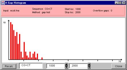
Figure 16. A gap length histogram.

The gap length histogram window has three major parts: the information bar on the top of the window, the histogram on the middle of the window and the recalculation controls plus the close button on the bottom of the window.

The information bar lists the following facts:

• Input: the name of the input file the DNA or RNA data was loaded from,
• Sequence: the sub-sequence or the combination of sub-sequences connected by ‘+’ operator we are interested in,
• Method: the method used to visualize the data (gap hist = gap length histogram),
• Start loc: the start location (the position of the first base) of the interval we are scanning,
• Stop loc: the stop location (the position of the last base) of the interval we are scanning,
• Overflow gaps: the number of gaps that are wider than the widest gap visualized on the histogram.

Using the recalculation controls on the bottom of the window, the user can change the parameters of the histogram. The following parameters can be changed: the sub-sequence (or sub-sequences connected with ‘+’) of interest and the scanned interval of the DNA/RNA sequence. Press the recalculate button after adjusting the parameters to update the histogram.

5.6 Using projection curves

5.6.1 What is a projection curve ?

A projection curve is a graph describing the distribution of a sub-sequence along a DNA/RNA sequence. Instead of a gap length histogram that shows only frequency-counts of gaps, we actually see the location specific information about the occurrences of the sub-sequence.

The projection function f_p is a cumulative sum of +1 and –1. The idea behind the projection function is to scan over the DNA/RNA sequence base by base and if a hit of the sub-sequence is encountered +1 is added, otherwise –1 is added. So, in fact, the value of (f_p(x) | 1 £ x £ length of the DNA/RNA sequence) is the subtraction of those locations starting the sub-sequence and those locations not starting the sub-sequence inside the interval [1, x]. This method has been used in the literature to detect sub-sequences of biological significance, e.g., occurrence of C+G rich regions, location of the origin of replication in bacterial genome [3].

To see an example of a projection function, refer to the projection curve in the Figure 17.

5.6.2 A projection curve and GenPatterns

GenPatterns implements a tool to plot projection curves. The projection curve tool and the gap length histogram tool are located under the same sub-system: The Gap Plot Analyzer. To launch the Gap Plot Analyzer, select ‘Gap Plots…’ from the ‘Tools’ menu. Note, as with a gap length histogram, an actual DNA or RNA sequence (sample) is required to utilize the projection curve.

The dialog window of the Gap Plot Analyzer is shown in the Figure 15. The usage of the dialog window has already been described previously. To launch a projection curve window, select ‘Sub-sequence projection curve’ from ‘Select the type of the Gap Plot’. Refer to the section 5.4.2 to find the explanation of the fields on the gap plot analyzer - dialog window.

A window like the one in the Figure 17 is created to show a projection curve.

Figure 17. A projection curve window.

A projection curve window has three main parts: the information and control panel on the top of the window, the projection curve in the middle of the window and the recalculation controls plus the close button on the bottom of the window.

The information and control panel shows the following information:

• Input: the name of the input Fasta file the DNA/RNA data was loaded from,
• Method: the method used to visualize the data (proj curve = projection curve),
• Base: exact base number the mouse pointer is pointing to. This number changes as you move the mouse on the curve.

Additionally, the information and control panel includes the following controls:

· Add curve (button): add a new curve on top of the existing one. A new set of user interface components is added on the bottom of the window. The number of curves in a window is limited to at most three,

· Del curve (button): removes the curve added last,

· Vertical markers (check box): when checked, draws a vertical marker on those positions the projection curve function gets one added (an occurrence of a sub-sequence of interest). See Figure 18 for an example of a curve with vertical markers,

Figure 18. A projection curve of “CG” with vertical markers.

· Confidence interval (check box): when checked, draws the confidence interval on the projection curve window using the Z value from the Z field. A confidence interval is a notion from probability. For a given confidence level, it represents an interval a specified normally distributed random variable will fall within with the given level of confidence. In our case, it represents an interval the projection curve will fall within with the given level of confidence, stated by the Z value,

• Z (text field): enter the Z value used in the confidence interval calculations. The default value is 3, which represents approximately 99.5% confidence. Other common limits are Z = 1.96 (95%), Z = 2.58 (99%) and Z = 3.29 (99.9%).

Figure 19 shows a projection curve with a confidence interval and Figure 20 shows a projection curve window with two curves.

Figure 19. A projection curve window with a confidence interval.

Figure 20. A projection curve window with two curves.

The recalculation controls on the bottom of the window include a text field for every sub-sequence (or a combination of sub-sequences connected with ‘+’) following by a color bar indicating the color of the corresponding curve, the numeric spinner controls to change the sub-interval of interest in the DNA/RNA sequence and the Recalc –button, which is used to recalculate the curves using current parameters.

On the right side of the numeric spinners controlling the interval size and location, are two buttons, labeled as ‘>>’ and ‘<<’. These are quick controls to change the selected sub-interval. Pressing the ‘>>’ button, moves the window to the right by a window size. The ‘<<’ button, on the other hand, moves window to the left.

5.7 Using DNA walks

5.7.1 What is a DNA walk ?

The DNA walk is a method of visualizing the structural behavior of a DNA or RNA sequence. The DNA walk is a curve that takes a step to either left, right, up or down depending on each base of the DNA/RNA sequence. The curve is formed by scanning through the sequence and checking the sub-sequence(s) associated to each direction against each location on the DNA/RNA sequence. In the simplest case, each of the nucleotides A, C, G and T (U instead of T with RNA) are tied to a different direction, e.g., A=down, C=left, G=right and T=up. In this case each A on the sequence moves the curve one step down, C one step left, G one step right and T one step up.

More complex sub-sequence expressions can also be used instead of just simple nucleotides. For example, the following would be a possible combination with a DNA input: CT=down, (CGC or CGG)=left, (GCC or GCG)=right, AG=up. The expression (CGC or CGG)=left means that if either CGC or CGG starts from the DNA sequence position currently under interest the curve is moved one step left. If the current DNA sequence position starts a sub-sequence that is not associated to any directions, the curve is not advanced to any directions.

See the Figure 21 for an example of a DNA walk curve.

5.7.2 A DNA walk and GenPatterns

GenPatterns implements the DNA walk feature. Select “DNA Walk” from the “Tools” menu of the histogram window to launch a DNA Walk for the current input data. Note that a DNA Walk needs an actual DNA or RNA sequence so it doesn’t work with a Markov frequency-count model. The following figure shows an example of a DNA Walk of the Ecoli data.

Figure 21. A DNA Walk.

The beginning of the curve is indicated with a green box (on the top left corner in the example above) and the end of the curve is indicated with a red box (on the right in the example). The sub-sequence – direction –association is located in a different (dialog) window, which can be activated by moving the pointer on top of the pink area on top of the window. The following figure shows an example of that window.

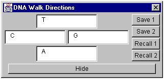
Figure 22. The DNA Walk DIrections window.

You can change the direction –sequence(s) associations using the DNA Walk Directions window. Just enter the sequence of interest in one of the direction fields on the window and press the “Recalc” button on the DNA Walk window. You can change any or all of the direction associations before pressing “Recalc”. Instead of just one sequence you can enter alternative sequences for one direction using the separator “+”. For example, CG+CC+CA means either CG or CC or CA.

Once you have entered new directions, you may wish to save them for use in another DNA walk, or for later use in this one. Simply press “Save 1” or “Save 2” to store the directions into one of two memory locations. After a set of directions has been saved, it can be recalled by pressing the Recall button that corresponds to the memory position the directions were saved in (1 or 2).

The DNA Walk curve in the Figure 21 shows the interval from the 1^st to 20000^th base. This interval can be changed either by entering new values for the value fields or by using quick controls, labeled “<<” and “>>”. Press the “>>” button to move the interval one “window” to the right (on the DNA/RNA sequence). The button “<<” moves the window to the left. After entering new interval limits press “Recalc” to recalculate (update) the curve.

A DNA Walk window has a controls field (colored pink) on top of the window (see Figure 21). The controls field has several information fields and controls. The ‘Input’ field gives the name of the input data file. ‘Length’ is the length of the input sequence. And ‘Incr. scale’ (Increment scale) is the number of DNA walk steps per pixel. It is important to understand the meaning of the increment scale. If the increment scale is, for example, 0.25, the DNA walk has to travel 4 steps to certain direction before the movement is shown on the screen. The following figure clarifies the situation.

Figure 23. The meaning of the Increment Scale value.

Note that the size of a DNA walk increment scale on the figure is 0.25 pixels and only those pixels visited by the curve are colored as a part of the curve on the screen.

It is possible to label the sequence positions along the curve on the screen. Check the “Base labels” checkbox to activate this feature. Under the checkbox is an input field of the size of a label interval on the screen (in base pairs). Enter a new value to either shrink or expand the interval.

As we already know, if the current DNA/RNA sequence position starts a sub-sequence that is not associated to any directions, the curve is not advanced to any directions. We have an optional feature to visualize these “stationary” positions on the curve. Check the “Gaps” checkbox to activate this feature. Every time the curve is not advanced, a circle is drawn around the current position of the curve. The current end of the curve is the center of the circle and the diameter of the circle is determined the following way: the more consecutive positions on the DNA/RNA sequence without an occurrence of the sub-sequence hit the bigger the diameter. To be more exact, the size of the diameter follows the formula gl*is, where ‘gl’ stands for the length of the gap in base pairs and ‘is’ is the increment scale value. The following figure shows an example of a DNA walk with the gap circles.

Figure 24. A DNA Walk with gap circles.

As you can see most of the time there are only small sections (gaps) on the DNA sequence (indicated by small blue circles) where none of the interesting sub-sequences is encountered. Only few exceptions are present, the most obvious being the big circle near the end of the sequence (the up-right corner). In the center of that circle lies the point of the curve where there is a wide section on the original DNA sequence with none of the sub-sequence of interest.

5.7.3 Double DNA walks

In a double DNA walk, two DNA walk curves are show in one window. The first curve is black, and the second curve is blue. To activate a double DNA walk, select “Double DNA Walk” from the tools menu. The resulting screen allows you to choose which DNA/file will be the first curve, and which will be the second curve. Both curves are allowed to be from the same source. This can be helpful if, for example, you want to view the beginning and end, but not the middle, of a DNA sequence, as shown in Figure 25. The portion of the sequence visualized can be set independently for each of the two curves. The two boxes on the top are for the first curve, and the two on the bottom are for the second curve. If RNA and DNA are in a double walk together, the RNA will interpret a T in the directions as a U, and the DNA will interpret a U in the directions at a T.

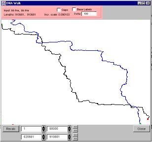
Figure 25. A Double DNA Walk

5.8 Modifying Histogram Properties

5.8.1 Changing the axes/ordering

By default, a histogram is sorted with the order GCAT. The user can change this order by selecting “Axes” from the Edit Menu. The resulting window is pictured in Figure 26.

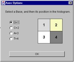
Figure 26: Changing the axes

First, select the base you want to move. (G is selected in Figure 26.) Then, click on the position the selected base should move to in the sample Hao histogram. The selected base will move to its new position, and the base previously occupying the position will take the selected base’s place in the order. Click “OK” to dismiss the dialog.

5.8.2 Changing the maximum level

It is possible to change the maximum level the program will calculate for a new histogram. Recall that frequencies are calculated for each ‘word’ up to the highest level. For example ATGCC, a five base word, would have a square representing its frequency displayed when the histogram is set at level five.

To change the level, click on the rectangle to the left of the buttons on the Control Panel, or select “Max Level” from the Edit menu of a histogram. Below the warnings is a box where the level can be changed. It cannot be set lower than one or higher than fifteen. The level set is used the next time a histogram is created. Histograms already created will not be affected. When a comparison histogram is created, its maximum level is the maximum level set or the maximum level of the histograms it is comparing, whichever is smaller.

Decreasing the maximum level will cause each newly created histogram to use less memory and to load faster. If the default is higher than is needed, decreasing it is encouraged.

Increasing the maximum level by one will cause each newly created histogram to use about four times as much memory. It will also cause the file to load slower. It is easy to run out of memory if the level is set too high, so increase it with caution. Section 4.1.1 ‘Standalone program’ explains how to increase the amount of memory available to GenPatterns.

6 References

[1] Hao B. et al, A Combinatorial Problem Related to Avoided and Under-Represented Strings in Bacterial Complete Genomes. Proc. of Combinatorics and Physics, Los Alamos, August 1998.

[2] Hunt F., Y., Pesonen A., GenPatterns – Program Description. NIST/ITL technical report, Gaithersburg, December 1999.

[3] Freeman J. et al, Patterns of Genome Organization in Bacteria. Science Magazine, Vol. 279, No. 5358, p.1827, 1998.

[4] Leong P., M., Morgenthaler S., Random walk and gap plots of DNA sequences. CABIOS, Vol. 11, no. 5, pp. 503 – 507, 1995.

[5] Gates M., A Simple Way to Look at DNA. J. Theor. Biol., Vol. 119, pp. 319 – 328, 1986.

Appendix: The applet restrictions

The applet version of GenPatterns is a demonstration of the "stand alone", Java coded, GenPatterns program. The applet version has some restrictions that are caused by the Internet browser security restrictions. The restrictions are listed and explained below:

• The following DNA example data are available:
• humanIe.fna (106 kb, Homo sapiens DNA sequence from PAC 747L4 on chromosome 1q23-24)
• yeastI.fna (229 kb, Saccharomyces cerevisiae chromosome I, complete chromosome sequence)
• myge.fna (576 kb, Mycoplasma genitalium, complete sequence)
• myp.fna (809 kb, Mycoplasma pneumoniae M129 complete genome)
• bb.fna (903 kb, Genomic sequence of a Lyme disease spirochete, Borrelia burgdorferi)
• moco.fna (192 kb, Molluscum contagiosum virus subtype 1, complete genome)
• mesa.fna (238 kb, Melanoplus sanguinipes entomopoxvirus, complete genome)

When the applet asks to enter an input file name, enter one of the names just listed. Use of only the data files provided by us is enforced by the fact that the applet enabled web browsers have security restriction, limiting the access to local resources (like files). There is a way to relax these restrictions but to keep things simple the current approach was selected (keep in mind also, that the "stand alone" version of GenPatterns does not have these limitations).

· File saving is disabled. Because of this, the color map changes are session specific and are not saved anywhere. Also, storing frequency files and file information files is disabled.