During the solidification of a pure material or an alloy, the crystalline solid often grows with a very complicated dendritic morphology. The so-called microstructure of the solid can be impacted by the nature of the dendritic growth process. In the last five years, computations of dendritic growth using the phase-field method have provided some of the most qualitatively realistic simulations of this highly complex phenomenon which involves an interplay between diffusion in the bulk phases and surface energy and kinetic effects at the solid/liquid interface. Simulations performed using numerical algorithms developed in the ACMD have provided a better understanding of the nature of the interaction between the various physical mechanisms and have allowed material scientists and physicists to test and modify existing simplified theories. Currently, it has been proposed to use the micro-scale study of dendritic growth via the phase-field computations to guide the development of meso-scale models which can then be employed in large-scale computations for the solidification of castings; casting simulations can reduce the development costs and improve the quality of cast parts.
The phase-field method introduces a continuous transition region between the two bulk phases (e.g., solid/liquid). This transition region is defined in terms of an additional field variable (the phase field), which is formulated to represent the dynamical evolution of the phase-change interface. In contrast, the classical free boundary approach models solidification by treating the solid and liquid phases individually and by explicitly determining the moving interface between the two bulk phases in order to apply the appropriate boundary conditions. At the cost of solving an additional partial differential equation, the advantage of the phase-field method is that the location of the interface does not have to be explicitly determined (or tracked) as part of the solution.
While the phase-field technique offers considerable promise for phase-change computations, it has become evident that adaptive solution techniques will be necessary in order to treat the conditions of relevant experiments (3-D and low undercooling) and for practical applications. Recent work in ACMD involves adapting a general purpose adaptive finite-difference algorithm to solve the phase-field equations for the solidification of a pure material in two-dimensions. The algorithm uses uniform mesh refinement in regions with steep gradients of the solution variables. Computations have been successfully performed employing up to four refinement levels. The efficiency and accuracy of the adaptive computations are presently being compared to the fixed grid solutions developed in ACMD for the phase-field equations.
As an example of the adaptive phase-field simulations, displayed below, shows a single solid dendrite growing into an undercooled liquid (below the freezing temperature) at an early time in the computation. The top half of the figure shows two branches of the dendrite growing along the axes. The interfacial region is displayed by three contour lines. The solid region is below and to the left of the interface; above and to the right is undercooled liquid. The dendritic image has been reflected in the bottom half of the figure. Superimposed on the phase-field contours are the refinement regions. The base (coarse) mesh comprises most of the domain outside of the widest demarcation lines around the interface. Successively closer lines mark the three refined regions closer to the interface.
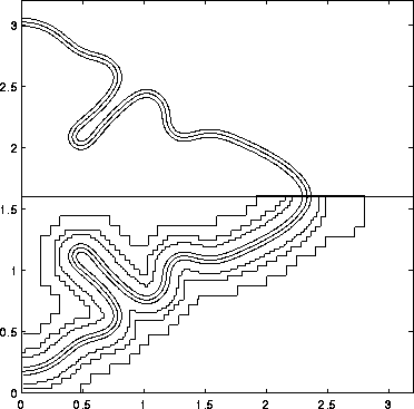
Caption: Adaptive mesh phase-field computations of a growing dendrite into an undercooled liquid. The top-half shows only the growing solid which is outlined by three contours of the phase-field variable marking the interfacial region. The bottom half has the outline of the grid refinement regions superimposed.